Multiple Regression
Functions:
Multiple regression allows us to see the relationship between two variables, accounting for other variables in the model.
We will use the state.x77 dataset included with R.
It is a matrix with 50 rows and 8 columns giving the following statistics in the respective columns.
Population: population estimate as of July 1, 1975.
Income: per capita income (1974)
Illiteracy: illiteracy (1970, percent of population)
Life Exp: life expectancy in years (1969-71)
Murder: murder and non-negligent manslaughter rate per 100,000 population (1976)
HS Grad: percent high-school graduates (1970)
Frost: mean number of days with minimum temperature below freezing (1931-1960) in capital or large city
Area: land area in square miles
Source: U.S. Department of Commerce, Bureau of the Census (1977) Statistical Abstract of the United States, and U.S. Department of Commerce, Bureau of the Census (1977) County and City Data Book.
# load the data
data(state)
state.x77
## Population Income Illiteracy Life Exp Murder HS Grad Frost
## Alabama 3615 3624 2.1 69.05 15.1 41.3 20
## Alaska 365 6315 1.5 69.31 11.3 66.7 152
## Arizona 2212 4530 1.8 70.55 7.8 58.1 15
## Arkansas 2110 3378 1.9 70.66 10.1 39.9 65
## California 21198 5114 1.1 71.71 10.3 62.6 20
## Colorado 2541 4884 0.7 72.06 6.8 63.9 166
## Connecticut 3100 5348 1.1 72.48 3.1 56.0 139
## Delaware 579 4809 0.9 70.06 6.2 54.6 103
## Florida 8277 4815 1.3 70.66 10.7 52.6 11
## Georgia 4931 4091 2.0 68.54 13.9 40.6 60
## Hawaii 868 4963 1.9 73.60 6.2 61.9 0
## Idaho 813 4119 0.6 71.87 5.3 59.5 126
## Illinois 11197 5107 0.9 70.14 10.3 52.6 127
## Indiana 5313 4458 0.7 70.88 7.1 52.9 122
## Iowa 2861 4628 0.5 72.56 2.3 59.0 140
## Kansas 2280 4669 0.6 72.58 4.5 59.9 114
## Kentucky 3387 3712 1.6 70.10 10.6 38.5 95
## Louisiana 3806 3545 2.8 68.76 13.2 42.2 12
## Maine 1058 3694 0.7 70.39 2.7 54.7 161
## Maryland 4122 5299 0.9 70.22 8.5 52.3 101
## Massachusetts 5814 4755 1.1 71.83 3.3 58.5 103
## Michigan 9111 4751 0.9 70.63 11.1 52.8 125
## Minnesota 3921 4675 0.6 72.96 2.3 57.6 160
## Mississippi 2341 3098 2.4 68.09 12.5 41.0 50
## Missouri 4767 4254 0.8 70.69 9.3 48.8 108
## Montana 746 4347 0.6 70.56 5.0 59.2 155
## Nebraska 1544 4508 0.6 72.60 2.9 59.3 139
## Nevada 590 5149 0.5 69.03 11.5 65.2 188
## New Hampshire 812 4281 0.7 71.23 3.3 57.6 174
## New Jersey 7333 5237 1.1 70.93 5.2 52.5 115
## New Mexico 1144 3601 2.2 70.32 9.7 55.2 120
## New York 18076 4903 1.4 70.55 10.9 52.7 82
## North Carolina 5441 3875 1.8 69.21 11.1 38.5 80
## North Dakota 637 5087 0.8 72.78 1.4 50.3 186
## Ohio 10735 4561 0.8 70.82 7.4 53.2 124
## Oklahoma 2715 3983 1.1 71.42 6.4 51.6 82
## Oregon 2284 4660 0.6 72.13 4.2 60.0 44
## Pennsylvania 11860 4449 1.0 70.43 6.1 50.2 126
## Rhode Island 931 4558 1.3 71.90 2.4 46.4 127
## South Carolina 2816 3635 2.3 67.96 11.6 37.8 65
## South Dakota 681 4167 0.5 72.08 1.7 53.3 172
## Tennessee 4173 3821 1.7 70.11 11.0 41.8 70
## Texas 12237 4188 2.2 70.90 12.2 47.4 35
## Utah 1203 4022 0.6 72.90 4.5 67.3 137
## Vermont 472 3907 0.6 71.64 5.5 57.1 168
## Virginia 4981 4701 1.4 70.08 9.5 47.8 85
## Washington 3559 4864 0.6 71.72 4.3 63.5 32
## West Virginia 1799 3617 1.4 69.48 6.7 41.6 100
## Wisconsin 4589 4468 0.7 72.48 3.0 54.5 149
## Wyoming 376 4566 0.6 70.29 6.9 62.9 173
## Area
## Alabama 50708
## Alaska 566432
## Arizona 113417
## Arkansas 51945
## California 156361
## Colorado 103766
## Connecticut 4862
## Delaware 1982
## Florida 54090
## Georgia 58073
## Hawaii 6425
## Idaho 82677
## Illinois 55748
## Indiana 36097
## Iowa 55941
## Kansas 81787
## Kentucky 39650
## Louisiana 44930
## Maine 30920
## Maryland 9891
## Massachusetts 7826
## Michigan 56817
## Minnesota 79289
## Mississippi 47296
## Missouri 68995
## Montana 145587
## Nebraska 76483
## Nevada 109889
## New Hampshire 9027
## New Jersey 7521
## New Mexico 121412
## New York 47831
## North Carolina 48798
## North Dakota 69273
## Ohio 40975
## Oklahoma 68782
## Oregon 96184
## Pennsylvania 44966
## Rhode Island 1049
## South Carolina 30225
## South Dakota 75955
## Tennessee 41328
## Texas 262134
## Utah 82096
## Vermont 9267
## Virginia 39780
## Washington 66570
## West Virginia 24070
## Wisconsin 54464
## Wyoming 97203The data is currently a matrix
is.matrix(state.x77)## [1] TRUEstr(state.x77)## num [1:50, 1:8] 3615 365 2212 2110 21198 ...
## - attr(*, "dimnames")=List of 2
## ..$ : chr [1:50] "Alabama" "Alaska" "Arizona" "Arkansas" ...
## ..$ : chr [1:8] "Population" "Income" "Illiteracy" "Life Exp" ...So, let's make it into a dataframe
dat <- as.data.frame(state.x77)
head(dat)
## Population Income Illiteracy Life Exp Murder HS Grad Frost
## Alabama 3615 3624 2.1 69.05 15.1 41.3 20
## Alaska 365 6315 1.5 69.31 11.3 66.7 152
## Arizona 2212 4530 1.8 70.55 7.8 58.1 15
## Arkansas 2110 3378 1.9 70.66 10.1 39.9 65
## California 21198 5114 1.1 71.71 10.3 62.6 20
## Colorado 2541 4884 0.7 72.06 6.8 63.9 166
## Area
## Alabama 50708
## Alaska 566432
## Arizona 113417
## Arkansas 51945
## California 156361
## Colorado 103766We first need to fix a few things: removing spaces in variable names, and calculating the population density.
Spaces in column names work if you use [ to refer to columns, but not if you use $:
#head(dat['Life Exp'])

#head(dat$Life Exp)

# correct column names
colnames(dat)[4] <- "Life.Exp"
colnames(dat)[6] <- "HS.Grad"

# calculate density
dat$Density <- dat$Population * 1000 / dat$Area
First, let's look at the relationships among all the variables.
plot(dat)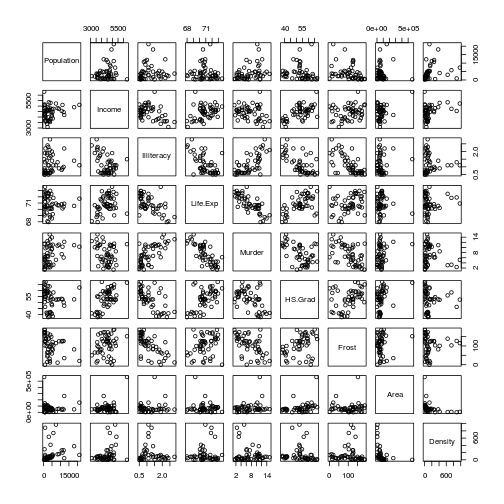
plot of chunk state-plot
Some of these look correlated. Let's check, calculating the correlation coefficients for each pairwise comparison.
cor(dat)## Population Income Illiteracy Life.Exp Murder
## Population 1.00000000 0.2082276 0.107622373 -0.06805195 0.3436428
## Income 0.20822756 1.0000000 -0.437075186 0.34025534 -0.2300776
## Illiteracy 0.10762237 -0.4370752 1.000000000 -0.58847793 0.7029752
## Life.Exp -0.06805195 0.3402553 -0.588477926 1.00000000 -0.7808458
## Murder 0.34364275 -0.2300776 0.702975199 -0.78084575 1.0000000
## HS.Grad -0.09848975 0.6199323 -0.657188609 0.58221620 -0.4879710
## Frost -0.33215245 0.2262822 -0.671946968 0.26206801 -0.5388834
## Area 0.02254384 0.3633154 0.077261132 -0.10733194 0.2283902
## Density 0.24622789 0.3299683 0.009274348 0.09106176 -0.1850352
## HS.Grad Frost Area Density
## Population -0.09848975 -0.332152454 0.02254384 0.246227888
## Income 0.61993232 0.226282179 0.36331544 0.329968277
## Illiteracy -0.65718861 -0.671946968 0.07726113 0.009274348
## Life.Exp 0.58221620 0.262068011 -0.10733194 0.091061763
## Murder -0.48797102 -0.538883437 0.22839021 -0.185035233
## HS.Grad 1.00000000 0.366779702 0.33354187 -0.088367214
## Frost 0.36677970 1.000000000 0.05922910 0.002276734
## Area 0.33354187 0.059229102 1.00000000 -0.341388515
## Density -0.08836721 0.002276734 -0.34138851 1.000000000For now, let's assume that all these variables are not sufficiently correlated to prohibit our analysis.
We might construct a model of life expectancy as a function of all the other variables (we could come up with reasonable hypotheses that that population size and density, income levels, illiteracy and murder rates, education and climate all might influence mean life expectancy).
We run a full model.. a model with all the variables.
m.full <- lm(Life.Exp ~ Population + Income + Illiteracy + Murder + HS.Grad + Frost + Area + Density, data = dat)
summary(m.full)
##
## Call:
## lm(formula = Life.Exp ~ Population + Income + Illiteracy + Murder +
## HS.Grad + Frost + Area + Density, data = dat)
##
## Residuals:
## Min 1Q Median 3Q Max
## -1.47514 -0.45887 -0.06352 0.59362 1.21823
##
## Coefficients:
## Estimate Std. Error t value Pr(>|t|)
## (Intercept) 6.995e+01 1.843e+00 37.956 < 2e-16 ***
## Population 6.480e-05 3.001e-05 2.159 0.0367 *
## Income 2.701e-04 3.087e-04 0.875 0.3867
## Illiteracy 3.029e-01 4.024e-01 0.753 0.4559
## Murder -3.286e-01 4.941e-02 -6.652 5.12e-08 ***
## HS.Grad 4.291e-02 2.332e-02 1.840 0.0730 .
## Frost -4.580e-03 3.189e-03 -1.436 0.1585
## Area -1.558e-06 1.914e-06 -0.814 0.4205
## Density -1.105e-03 7.312e-04 -1.511 0.1385
## ---
## Signif. codes: 0 '***' 0.001 '**' 0.01 '*' 0.05 '.' 0.1 ' ' 1
##
## Residual standard error: 0.7337 on 41 degrees of freedom
## Multiple R-squared: 0.7501, Adjusted R-squared: 0.7013
## F-statistic: 15.38 on 8 and 41 DF, p-value: 3.787e-10Note: Running a multiple regression really is different from running lots of simple (single) regressions. Compare the coefficients for poplation in this simple regression with that above.
m0 <- lm(Life.Exp ~ Population, data = dat)
summary(m0)
##
## Call:
## lm(formula = Life.Exp ~ Population, data = dat)
##
## Residuals:
## Min 1Q Median 3Q Max
## -2.94787 -0.74453 -0.09087 1.09220 2.65227
##
## Coefficients:
## Estimate Std. Error t value Pr(>|t|)
## (Intercept) 7.097e+01 2.654e-01 267.409 <2e-16 ***
## Population -2.046e-05 4.330e-05 -0.473 0.639
## ---
## Signif. codes: 0 '***' 0.001 '**' 0.01 '*' 0.05 '.' 0.1 ' ' 1
##
## Residual standard error: 1.353 on 48 degrees of freedom
## Multiple R-squared: 0.004631, Adjusted R-squared: -0.01611
## F-statistic: 0.2233 on 1 and 48 DF, p-value: 0.6387Here, in model m0, we are not accounting for all the other variables. The effect size of population is quite different, and the direction of the relationship is opposite!
Interpreting the results
What do these results mean?
In contrast to the ANCOVA, we have no categorical variables. Thus, all the coefficients presented (apart from line 1) are slopes and we do not need to do any calculations to work out the actual effect sizes.
Each estimate is the change in y for a change in 1 unit of x. This understanding makes more sense of the estimates. For example, the effect of population size on life expectancy looks very very small (6.480e-05 = 0.0000648 years). But this is for an increase of 1 person in the population.
It might be better to rescale the predictor variables, so that we can make more realistic comparisons among them (we will do this later).
For now, it looks like population and murder rates have significant effects on life expectancy.
We will leave this model as is for now. Many non-statisticians will proceed to try and simplify this model to get only predictors with significant p-values. We will look at why this is a bad idea later.
Plotting the results
There are two ways to present results. We could basically copy the results into a table. Or, we could make a nice figure that allows us to easily compare effect sizes.
There are a number of simple steps to this.
First, we make an easier table of the values we are interested in using summary(m.full$coeff). We do not need to plot the intercept (line 1), so we remove this using indexing. Making this into a data frame allows us to access the columns as normal.
res <- as.data.frame(summary(m.full)$coef[-1, ])

# Change names because of spaces
names(res) <- c('Estimate', 'Std.Error', 't.value', 'P')
We could plot each line in order, as follows.
plot(res$Estimate)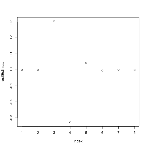
plot of chunk full-basic
But this is not very helpful for plotting the variable names, etc, so we will flip it and extend the x axes to accommodate any error bars.
# ensure that y-margins are large enough for labels
par(mar = c(4,7, 2, 2), lwd = 2)

# plot data in order
plot(1:8 ~ res$Estimate,
     xlim = c(-0.5, 0.5), xlab = 'Estimate',
     yaxt = 'n', ylab = '')

# add zero line
abline(v = 0, lty = 3, col = 'grey')


# add axis to side 2
axis(side = 2, at = 1:8, labels = rownames(res), las = 1)

# Then we can add the error bars, using ```segments()``` as before.
# standard error
segments(x0 = res$Estimate - res$Std.Error, x1 = res$Estimate + res$Std.Error,
         y0 = 1:8, y1 = 1:8)


# Finally, we can color each point depending on whether is has a significant p-value.
COL <- c('white', 'black')
points(x = res$Estimate, y = 1:8, pch = 21, cex = 2,
       bg = COL[(res$P < 0.05)+1])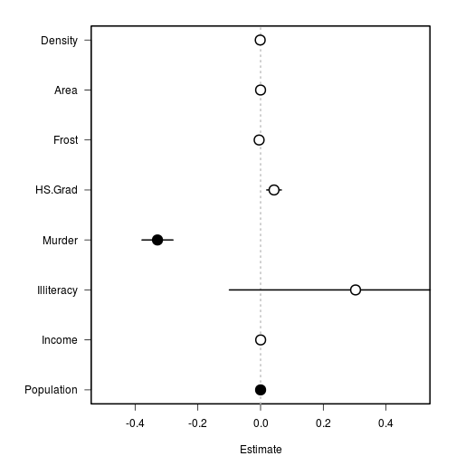
plot of chunk m.full-figure
Now we can easily see which variables are significant and how they compare.
Updated: 2017-11-03