Including Multiple Predictor Variables in Models
Functions: coef(), summary.lm(),
In the ANOVA and simple regression models that we have run so far, most of them have been a single response/dependent variable as a function of a single predictor/independent variable. But in many cases we know that there are several things that could reasonably influence the response variable. For example, species and sex could both affect sparrow size; age and sex could both influence running time.
It is straightforward to include multiple predictors. We start with the simple, special case of Analysis of Covariance (ANCOVA).
Analysis of Covariance
Statisticians realised early on that ANOVA was merely the beginning of analysing experiments---other factors apart from the experimental treatment might influence the response variable they were interested in. This issue is especially pertinent when considering change, i.e., does our experimental treatment affect growth or survival? The starting point of each sample is important. If we are measuring growth of seedlings, how big that seedling is at the start of the experiment will have a big affect on its growth. Moreover, if by chance all the big seedlings ended up in one treatment and the small ones in another, we may erroneously assign significance to the treatment.
Thus, analysis of variance with a continuous covariate was born, and we can ask if our treatment had a significant effect, accounting for the measured variation in seedling initial size, for example.
We can illustrate with the sparrow data,
#dat <- read.table(file = "http://www.simonqueenborough.info/R/data/sparrows.txt", header = TRUE)
dat <- read.table('~/Dropbox/MyLab/website/R/data/sparrows.txt', header = TRUE, sep = '\t')
and ask if male sparrows tend to have larger heads than female sparrows.
stripchart(dat$Head~dat$Sex, vertical = TRUE, method = 'jitter', col = c('darkgrey', 'red'), pch = 21)
points(x = 1:2, y = tapply(dat$Head, dat$Sex, mean), pch = 20, cex = 2)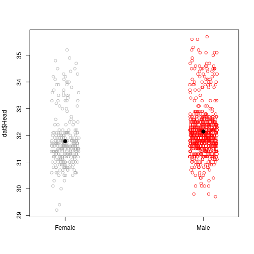
Fig. sparrow heads.
summary(aov(Head ~ Sex, data = dat))## Df Sum Sq Mean Sq F value Pr(>F)
## Sex 1 26.9 26.922 30.2 4.98e-08 ***
## Residuals 977 871.0 0.892
## ---
## Signif. codes: 0 '***' 0.001 '**' 0.01 '*' 0.05 '.' 0.1 ' ' 1However, we can reasonably assume that larger sparrows in general will have larger heads. Accounting for sparrow size as we compare sex might be a good idea.
We can include a different measure of sparrow size, such as Tarsus length, in the model. A plot of these data looks like this.
par(mfrow = c(1,2))

stripchart(dat$Head~dat$Sex, vertical = TRUE, method = 'jitter', col = c('darkgrey', 'red'), pch = 21)
points(x = 1:2, y = tapply(dat$Head, dat$Sex, mean), pch = 20, cex = 2)

plot(Head ~ Tarsus, data = dat[dat$Sex == 'Female', ], pch = 21)
points(Head ~ jitter(Tarsus), data = dat[dat$Sex == 'Male',] , col = 'red', pch = 21)
legend('topleft', pch = c(21, 21), col = c(1,2), legend = c('Female', 'Male'))
Fig. Including Tarsus
First, the simplest, additive, model. This examines the effect of Tarsus size on Head size, then tests whether each sex has a different relationship (i.e., the two sexes have different intercepts).
m0 <- aov(Head ~ Tarsus + Sex, data = dat)
summary(m0)
## Df Sum Sq Mean Sq F value Pr(>F)
## Tarsus 1 434 434.0 912.863 <2e-16 ***
## Sex 1 0 0.0 0.001 0.978
## Residuals 976 464 0.5
## ---
## Signif. codes: 0 '***' 0.001 '**' 0.01 '*' 0.05 '.' 0.1 ' ' 1Note that we put the continuous covariate (Tarsus) first in the model formula, before the factor (Sex). This is because R conducts the ANOVA tests sequentially, thus removing (or accounting) for the effect of Tarsus before testing for differences between the sexes.
Compare the ANOVA output to the alternative way of specifying the model.
m1 <- aov(Head ~ Sex + Tarsus, data = dat)
summary(m1)
## Df Sum Sq Mean Sq F value Pr(>F)
## Sex 1 26.9 26.9 56.63 1.19e-13 ***
## Tarsus 1 407.0 407.0 856.23 < 2e-16 ***
## Residuals 976 464.0 0.5
## ---
## Signif. codes: 0 '***' 0.001 '**' 0.01 '*' 0.05 '.' 0.1 ' ' 1The order only affects the ANOVA table, not the linear model summary, both of which show that sex is not significant.
summary.lm(m0)##
## Call:
## aov(formula = Head ~ Tarsus + Sex, data = dat)
##
## Residuals:
## Min 1Q Median 3Q Max
## -2.49966 -0.42453 0.00034 0.42574 2.46084
##
## Coefficients:
## Estimate Std. Error t value Pr(>|t|)
## (Intercept) 16.552598 0.522026 31.708 <2e-16 ***
## Tarsus 0.721000 0.024640 29.261 <2e-16 ***
## SexMale 0.001364 0.049871 0.027 0.978
## ---
## Signif. codes: 0 '***' 0.001 '**' 0.01 '*' 0.05 '.' 0.1 ' ' 1
##
## Residual standard error: 0.6895 on 976 degrees of freedom
## Multiple R-squared: 0.4833, Adjusted R-squared: 0.4822
## F-statistic: 456.4 on 2 and 976 DF, p-value: < 2.2e-16summary.lm(m1)##
## Call:
## aov(formula = Head ~ Sex + Tarsus, data = dat)
##
## Residuals:
## Min 1Q Median 3Q Max
## -2.49966 -0.42453 0.00034 0.42574 2.46084
##
## Coefficients:
## Estimate Std. Error t value Pr(>|t|)
## (Intercept) 16.552598 0.522026 31.708 <2e-16 ***
## SexMale 0.001364 0.049871 0.027 0.978
## Tarsus 0.721000 0.024640 29.261 <2e-16 ***
## ---
## Signif. codes: 0 '***' 0.001 '**' 0.01 '*' 0.05 '.' 0.1 ' ' 1
##
## Residual standard error: 0.6895 on 976 degrees of freedom
## Multiple R-squared: 0.4833, Adjusted R-squared: 0.4822
## F-statistic: 456.4 on 2 and 976 DF, p-value: < 2.2e-16We can add in the interaction. This model tests not only for different intercepts (different Head size by Sex), but also different slopes (is the slope of Head ~ Tarsus different between males and females).
m2 <- aov(Head ~ Tarsus * Sex, data = dat)
summary(m2)
## Df Sum Sq Mean Sq F value Pr(>F)
## Tarsus 1 434.0 434.0 913.005 <2e-16 ***
## Sex 1 0.0 0.0 0.001 0.978
## Tarsus:Sex 1 0.5 0.5 1.153 0.283
## Residuals 975 463.4 0.5
## ---
## Signif. codes: 0 '***' 0.001 '**' 0.01 '*' 0.05 '.' 0.1 ' ' 1From the plots it looks unlikely that there are different slopes, and the interaction model confirms this.
Plotting the lines
First, previously when we used abline() to plot the fitted line of the simple regression, we entered the model object name as an argument. This worked in that case, because the model contained only one intercept and one slope. With two or more predictor variables, we need to be a bit more careful.
Second, we mentioned that ANOVA and linear regression are effectively one and the same. We can, therefore, view the results of an ANOVA both as a traditional ANOVA table:
summary(m1)## Df Sum Sq Mean Sq F value Pr(>F)
## Sex 1 26.9 26.9 56.63 1.19e-13 ***
## Tarsus 1 407.0 407.0 856.23 < 2e-16 ***
## Residuals 976 464.0 0.5
## ---
## Signif. codes: 0 '***' 0.001 '**' 0.01 '*' 0.05 '.' 0.1 ' ' 1And also as the results of a linear regression, using the summary.lm() function:
summary.lm(m2)##
## Call:
## aov(formula = Head ~ Tarsus * Sex, data = dat)
##
## Residuals:
## Min 1Q Median 3Q Max
## -2.49831 -0.42447 0.00169 0.43124 2.45326
##
## Coefficients:
## Estimate Std. Error t value Pr(>|t|)
## (Intercept) 15.72467 0.93116 16.887 <2e-16 ***
## Tarsus 0.76020 0.04404 17.260 <2e-16 ***
## SexMale 1.21537 1.13177 1.074 0.283
## Tarsus:SexMale -0.05705 0.05313 -1.074 0.283
## ---
## Signif. codes: 0 '***' 0.001 '**' 0.01 '*' 0.05 '.' 0.1 ' ' 1
##
## Residual standard error: 0.6894 on 975 degrees of freedom
## Multiple R-squared: 0.4839, Adjusted R-squared: 0.4823
## F-statistic: 304.7 on 3 and 975 DF, p-value: < 2.2e-16The linear model summary provides us with the actual coefficient estimates and requires some interpretation. We will go through each section in turn (because the output is a list, they can also all be called independently using $).
First, we see the model that we ran.
summary.lm(m2)$call## aov(formula = Head ~ Tarsus * Sex, data = dat)Second, a summary of the distribution of the residuals.
summary(summary.lm(m2)$residuals)## Min. 1st Qu. Median Mean 3rd Qu. Max.
## -2.49800 -0.42450 0.00169 0.00000 0.43120 2.45300Third, the table of coefficients
summary.lm(m2)$coef## Estimate Std. Error t value Pr(>|t|)
## (Intercept) 15.72466830 0.93115876 16.887204 2.557025e-56
## Tarsus 0.76019705 0.04404265 17.260476 1.861108e-58
## SexMale 1.21536938 1.13176733 1.073869 2.831473e-01
## Tarsus:SexMale -0.05705086 0.05313452 -1.073706 2.832201e-01This table shows the coefficient estimates, standard error, and the t values and associated p values for significance tests. The way that the coefficients and tests are presented are different between categorical and continuous variables.
In this case, the first row of the output shows the mean Head size of females ('female' comes before 'male' alphanumerically), identified as the 'Intercept'. The test is whether this is different from 0.
The next row shows the mean Head size of males, but as the difference between that of females and males. I.e., to obtain the actual mean value of male Heads, you need to add the estimate for males to the value for females: 15.725 + 1.215. The test is whether this is different from 0 (i.e., there is a difference between male and female mean Head size).
The third row of the output shows the slope of the continuous variable (Tarsus) for females (0.76). The test is whether this slope is different from 0.
The forth row again show the difference in the slope between males and females. The test is whether this difference is different from 0 (i.e., females and males have different slopes).
Finally, the output provides some details of the R2 values and ANOVA table (F, df, p).
So, one way to add a line for each sex is as follows. We can extract the intercept and slope for females and males and then pass these values to abline().
F_intercept <- coef(m2)['(Intercept)']
F_slope     <- coef(m2)['Tarsus']
F_line       <- c(F_intercept, F_slope)

M_intercept <- F_intercept + coef(m2)['SexMale']
M_slope     <- F_slope + coef(m2)['Tarsus:SexMale']
M_line      <- c(M_intercept, M_slope)

par(lwd = 2, las = 1)
plot(Head ~ Tarsus, data = dat[dat$Sex == 'Female', ], pch = 21)
points(Head ~ jitter(Tarsus), data = dat[dat$Sex == 'Male',] , col = 'red', pch = 21)
legend('topleft', pch = c(21, 21), col = c(1,2), legend = c('Female', 'Male'))
abline(F_line, col = 'black')
abline(M_line, col = 'red')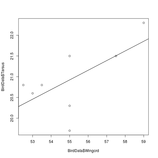
Fig. Head size in sparrows
Another way to obtain the fitted lines for each sex
We can modify the formula to return the actual coefficient estimates for each sex, rather than the differences (see formulas for more info on the kinds of formulas we can write).
First, we nest Tarsus in Sex: Sex/Tarsus. Then, we remove the single intercept using - 1.
m3 <- lm(Head ~ Sex/Tarsus - 1, data = dat)
summary(m3)
##
## Call:
## lm(formula = Head ~ Sex/Tarsus - 1, data = dat)
##
## Residuals:
## Min 1Q Median 3Q Max
## -2.49831 -0.42447 0.00169 0.43124 2.45326
##
## Coefficients:
## Estimate Std. Error t value Pr(>|t|)
## SexFemale 15.72467 0.93116 16.89 <2e-16 ***
## SexMale 16.94004 0.64330 26.33 <2e-16 ***
## SexFemale:Tarsus 0.76020 0.04404 17.26 <2e-16 ***
## SexMale:Tarsus 0.70315 0.02972 23.66 <2e-16 ***
## ---
## Signif. codes: 0 '***' 0.001 '**' 0.01 '*' 0.05 '.' 0.1 ' ' 1
##
## Residual standard error: 0.6894 on 975 degrees of freedom
## Multiple R-squared: 0.9995, Adjusted R-squared: 0.9995
## F-statistic: 5.288e+05 on 4 and 975 DF, p-value: < 2.2e-16This model gives us the actual intercepts and slopes for each sex. The p-values test whether each value is significantly different from 0 (not that useful).
Exercises
Examine the other variables in the large sparrow dataset. Are there differences in the relationships between two continuous variables depending on sex?
Quiz
The Orange dataset comes loaded in R. It describes the size (circumference) of five individual orange trees as a function of their age (age).
Load the data:
data(Orange)
head(Orange)
## Tree age circumference
## 1 1 118 30
## 2 1 484 58
## 3 1 664 87
## 4 1 1004 115
## 5 1 1231 120
## 6 1 1372 142# change the Tree levels to a simple factor
Orange$Tree <- factor(as.numeric(Orange$Tree))Plot circumference as a function of age, using different symbols or colors for each Tree.
Test for an effect of age on circumference.
Is this relationship the same for all Trees? Run a model to test this.
Add fitted lines for each Tree to the figure.
Updated: 2016-11-01