Linear Regression

Fitting a simple linear model

The maximum heart rate of a person is often said to be related to age by the equation

( Max = 220 - Age )

Age <- c(18, 23, 25, 35, 65, 54, 34, 56, 72, 19, 23, 42, 18, 39, 37)
Max.Rate <- c(202, 186, 187, 180, 156, 169, 174, 172, 153, 199, 193, 174, 198, 
    183, 178)

First, plot the data

plot(x = Age, y = Max.Rate)

plot of chunk heart

We use the linear model function lm() to fit linear models. At its simplest, it takes one argument: formula

lm(formula = Max.Rate ~ Age)

The response variable (Max.Rate) is fitted as a function of the predictor variable (Age). The tilde symbol (~) signifies as a function of, and separates the response and predictor variables. Adding further predictor variables to the right hand side is possible (see Formulae).

We can use the summary() function to look at the model output.

summary(lm(Max.Rate ~ Age))

We can also assign the linear model to another object, and use that instead. I tend to use m to signify a model.

m <- lm(Max.Rate ~ Age)
summary(m)

## 
## Call:
## lm(formula = Max.Rate ~ Age)
## 
## Residuals:
##    Min     1Q Median     3Q    Max 
## -8.926 -2.538  0.388  3.187  6.624 
## 
## Coefficients:
##             Estimate Std. Error t value Pr(>|t|)    
## (Intercept)  210.048      2.867    73.3  < 2e-16 ***
## Age           -0.798      0.070   -11.4  3.8e-08 ***
## ---
## Signif. codes:  0 '***' 0.001 '**' 0.01 '*' 0.05 '.' 0.1 ' ' 1
## 
## Residual standard error: 4.58 on 13 degrees of freedom
## Multiple R-squared:  0.909,  Adjusted R-squared:  0.902 
## F-statistic:  130 on 1 and 13 DF,  p-value: 3.85e-08

```

Adding a fitted line to a plot

we can use abline() to add the fitted line of the model to a plot of the raw data.

plot(Max.Rate ~ Age)
abline(lm(Max.Rate ~ Age))

plot of chunk heart2

Examining the model output

The output of lm() is similar to a list, and we can use the str() function to examine what is contained in the model output and see how to pull out certain parts of it.

str(m)

## List of 12
##  $ coefficients : Named num [1:2] 210.048 -0.798
##   ..- attr(*, "names")= chr [1:2] "(Intercept)" "Age"
##  $ residuals    : Named num [1:15] 6.31 -5.7 -3.11 -2.13 -2.2 ...
##   ..- attr(*, "names")= chr [1:15] "1" "2" "3" "4" ...
##  $ effects      : Named num [1:15] -698.17 -52.2 -3.63 -3.57 -6.41 ...
##   ..- attr(*, "names")= chr [1:15] "(Intercept)" "Age" "" "" ...
##  $ rank         : int 2
##  $ fitted.values: Named num [1:15] 196 192 190 182 158 ...
##   ..- attr(*, "names")= chr [1:15] "1" "2" "3" "4" ...
##  $ assign       : int [1:2] 0 1
##  $ qr           :List of 5
##   ..$ qr   : num [1:15, 1:2] -3.873 0.258 0.258 0.258 0.258 ...
##   .. ..- attr(*, "dimnames")=List of 2
##   .. .. ..$ : chr [1:15] "1" "2" "3" "4" ...
##   .. .. ..$ : chr [1:2] "(Intercept)" "Age"
##   .. ..- attr(*, "assign")= int [1:2] 0 1
##   ..$ qraux: num [1:2] 1.26 1.16
##   ..$ pivot: int [1:2] 1 2
##   ..$ tol  : num 1e-07
##   ..$ rank : int 2
##   ..- attr(*, "class")= chr "qr"
##  $ df.residual  : int 13
##  $ xlevels      : Named list()
##  $ call         : language lm(formula = Max.Rate ~ Age)
##  $ terms        :Classes 'terms', 'formula' length 3 Max.Rate ~ Age
##   .. ..- attr(*, "variables")= language list(Max.Rate, Age)
##   .. ..- attr(*, "factors")= int [1:2, 1] 0 1
##   .. .. ..- attr(*, "dimnames")=List of 2
##   .. .. .. ..$ : chr [1:2] "Max.Rate" "Age"
##   .. .. .. ..$ : chr "Age"
##   .. ..- attr(*, "term.labels")= chr "Age"
##   .. ..- attr(*, "order")= int 1
##   .. ..- attr(*, "intercept")= int 1
##   .. ..- attr(*, "response")= int 1
##   .. ..- attr(*, ".Environment")=<environment: R_GlobalEnv> 
##   .. ..- attr(*, "predvars")= language list(Max.Rate, Age)
##   .. ..- attr(*, "dataClasses")= Named chr [1:2] "numeric" "numeric"
##   .. .. ..- attr(*, "names")= chr [1:2] "Max.Rate" "Age"
##  $ model        :'data.frame':   15 obs. of  2 variables:
##   ..$ Max.Rate: num [1:15] 202 186 187 180 156 169 174 172 153 199 ...
##   ..$ Age     : num [1:15] 18 23 25 35 65 54 34 56 72 19 ...
##   ..- attr(*, "terms")=Classes 'terms', 'formula' length 3 Max.Rate ~ Age
##   .. .. ..- attr(*, "variables")= language list(Max.Rate, Age)
##   .. .. ..- attr(*, "factors")= int [1:2, 1] 0 1
##   .. .. .. ..- attr(*, "dimnames")=List of 2
##   .. .. .. .. ..$ : chr [1:2] "Max.Rate" "Age"
##   .. .. .. .. ..$ : chr "Age"
##   .. .. ..- attr(*, "term.labels")= chr "Age"
##   .. .. ..- attr(*, "order")= int 1
##   .. .. ..- attr(*, "intercept")= int 1
##   .. .. ..- attr(*, "response")= int 1
##   .. .. ..- attr(*, ".Environment")=<environment: R_GlobalEnv> 
##   .. .. ..- attr(*, "predvars")= language list(Max.Rate, Age)
##   .. .. ..- attr(*, "dataClasses")= Named chr [1:2] "numeric" "numeric"
##   .. .. .. ..- attr(*, "names")= chr [1:2] "Max.Rate" "Age"
##  - attr(*, "class")= chr "lm"

More explicitly, the result of lm() is of class lm and so the generic functions plot() and summary() commands adapt themselves to that. The variable lm.result contains the result.

We used summary() to view the entire thing. To view parts of it, you can call it like it is a list or better still use the following methods: resid() for residuals, coef() for coefficients and predict() for prediction.

Here are a few examples, the former giving the coefficients b0 and b1, the latter returning the residuals which are then summarized.

coef(m)

## (Intercept)         Age 
##    210.0485     -0.7977


coef(m)[1]

## (Intercept) 
##         210


summary(resid(m))

##    Min. 1st Qu.  Median    Mean 3rd Qu.    Max. 
##  -8.930  -2.540   0.388   0.000   3.190   6.620

Once we know the model is appropriate for the data, we can begin to identify the meaning of the numbers.

Testing the assumptions of the model

The lm() functios assumes that errors are INDEPENDENT AND IDENTICALLY DISTRIBUTED (i.i.d.) NORMAL RANDOM variables

We can test for normality with: histograms, boxplots and normal plots.
We can test for correlations by looking if there are trends in the data.
This can be done with plots of the residuals vs. time and order.
We can test the assumption that the errors have the same variance with plots of residuals vs. time order and fitted values.

The plot() command will do these tests for us if we give it the result of the regression. Note that the output is different from plot(y ~ x).

par(mfrow = c(2, 2))
plot(m)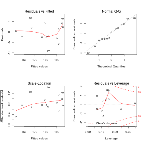

plot of chunk heart3

Residuals vs. fitted This plots the fitted y.hat values against the residuals. Look for spread around the line y = 0 and no obvious trend.

Normal qqplot The residuals are normal if this graph falls close to a straight line.

Scale-Location This plot shows the square root of the standardized residuals. The tallest points, are the largest residuals.

Cook's distance This plot identifies points which have a lot of influence in the regression line.

Statistical inference

If you are satisfied that the model fits the data, then statistical inferences can be made. There are 3 parameters in the model: sigma, beta0 and beta1.

sigma

Sigma is the standard deviation of the error terms. If we had the exact regression line, then the error terms and the residuals would be the same, so we expect the residuals to tell us about the value of sigma.

beta1

The estimator b1 for beta1, the slope of the regression line, is also an unbiased estimator.

R will automatically do a hypothesis test for the assumption beta1 = 0 which means no slope. The p-value is included in the output of the summary command in the column Pr(>|t|).

beta0

As well, a statistical test for b0 can be made (and is). Again, R includes the test for beta0 = 0 which tests to see if the line goes through the origin. Other tests are possible.

Predicted values

We can use the predict() function to get predicted values. We need a data frame with column names matching the predictor or explanatory variable.

In this example this is 'Age' so to get a prediction for a 50 and 60 year old we run:

predict(object = m, newdata = data.frame(Age = c(50, 60)) )

Confidence intervals

The regression line is used to predict the value of y for a given x, or the average value of y for a given x; but we also want to know how accurate this prediction is. This is the job of a confidence interval.

using predict()

predict(m, data.frame(Age = sort(Age)), level = 0.95, interval = "confidence")

##      fit   lwr   upr
## 1  195.7 191.8 199.6
## 2  195.7 191.8 199.6
## 3  194.9 191.1 198.7
## 4  191.7 188.4 195.0
## 5  191.7 188.4 195.0
## 6  190.1 186.9 193.3
## 7  182.9 180.3 185.5
## 8  182.1 179.6 184.7
## 9  180.5 178.0 183.1
## 10 178.9 176.4 181.5
## 11 176.5 173.9 179.2
## 12 167.0 163.4 170.6
## 13 165.4 161.6 169.2
## 14 158.2 153.3 163.1
## 15 152.6 146.8 158.4

Three numbers are returned for each value of x. (note we sorted x first to get the proper order for plotting.)

To plot the lower band, we just need the second column which is accessed with [,2]. So the following will plot just the lower. We can use points() or lines() to plot the intervals.

plot(Age, Max.Rate)
abline(m)
ci.lwr <- predict(m, data.frame(Age = sort(Age)), level = 0.95, interval = "confidence")[, 
    2]
points(sort(Age), ci.lwr, type = "l", lty = 3)

ci.upr <- predict(m, data.frame(Age = sort(Age)), level = 0.95, interval = "confidence")[, 
    3]
points(sort(Age), ci.upr, type = "l", lty = 3)

plot of chunk heart4

Exercises