ANOVA

One-way anova: aov()

A t-test is used to test hypotheses about the means of two independent samples, for example, to test if there is a difference between control and treatment groups. Two compare more than two independent samples, analysis of variance (ANOVA) is used.

x = c(4, 3, 4, 5, 2, 3, 4, 5)
y = c(4, 4, 5, 5, 4, 5, 4, 4)
z = c(3, 4, 2, 4, 5, 5, 4, 4)
scores = data.frame(x, y, z)
boxplot(scores)

Fig. Boxplot of means

Analysis of variance allows us to investigate if x, y, and z have the same mean. The R function to do the analysis of variance hypothesis test (oneway.test()) requires the data to be in a different format. It wants to have the data with a single variable holding the scores, and a factor describing the grader or category. The stack() command will do this for us:

scores = stack(scores)  # look at scores if not clear
names(scores)

## [1] "values" "ind"

head(scores)

##   values ind
## 1      4   x
## 2      3   x
## 3      4   x
## 4      5   x
## 5      2   x
## 6      3   x

Run the anova using aov()

m <- aov(values ~ ind, data = scores)
summary(m)

##             Df Sum Sq Mean Sq F value Pr(>F)
## ind          2   1.75   0.875    1.13   0.34
## Residuals   21  16.25   0.774



### Non-parametric anova: kruskal-wallis()

kruskal.test(values ~ ind, data = scores)

## 
##  Kruskal-Wallis rank sum test
## 
## data:  values by ind
## Kruskal-Wallis chi-squared = 1.939, df = 2, p-value = 0.3793

Two-way anova

For two independent predictor variables.

data

gr <- read.table("../data/growth.txt", header = T)

Plot the data.

tapply(gr$gain, list(gr$diet, gr$supplement), mean)

##        agrimore control supergain supersupp
## barley    26.35   23.30     22.47     25.58
## oats      23.30   20.49     19.66     21.86
## wheat     19.64   17.41     17.01     19.67

barplot(tapply(gr$gain, list(gr$diet, gr$supplement), mean), beside = TRUE, 
    ylim = c(0, 30), col = rainbow(3))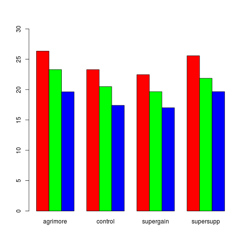

Fig. Growth by diet and supplement

Run the full interaction model

model <- aov(gain ~ diet * supplement, data = gr)
summary(model)

##                 Df Sum Sq Mean Sq F value Pr(>F)    
## diet             2  287.2   143.6   83.52  3e-14 ***
## supplement       3   91.9    30.6   17.81  3e-07 ***
## diet:supplement  6    3.4     0.6    0.33   0.92    
## Residuals       36   61.9     1.7                   
## ---
## Signif. codes:  0 '***' 0.001 '**' 0.01 '*' 0.05 '.' 0.1 ' ' 1

Run the simpler additive model.

model2 <- aov(gain ~ diet + supplement, data = gr)
summary.lm(model2)

## 
## Call:
## aov(formula = gain ~ diet + supplement, data = gr)
## 
## Residuals:
##     Min      1Q  Median      3Q     Max 
## -2.3079 -0.8593 -0.0771  0.9205  2.9061 
## 
## Coefficients:
##                     Estimate Std. Error t value Pr(>|t|)    
## (Intercept)           26.123      0.441   59.26  < 2e-16 ***
## dietoats              -3.093      0.441   -7.02  1.4e-08 ***
## dietwheat             -5.990      0.441  -13.59  < 2e-16 ***
## supplementcontrol     -2.697      0.509   -5.30  4.0e-06 ***
## supplementsupergain   -3.381      0.509   -6.64  4.7e-08 ***
## supplementsupersupp   -0.727      0.509   -1.43     0.16    
## ---
## Signif. codes:  0 '***' 0.001 '**' 0.01 '*' 0.05 '.' 0.1 ' ' 1
## 
## Residual standard error: 1.25 on 42 degrees of freedom
## Multiple R-squared:  0.853,  Adjusted R-squared:  0.836 
## F-statistic: 48.8 on 5 and 42 DF,  p-value: <2e-16

We can examine the model in two ways.

To return an ANOVA table, use aov() and summary().
To return coefficient estimates, use aov() and summary.lm(); or lm() and summary().

We can also use the anova() function to compare the two models, and test for a significant difference between them. Which model is better?

anova(model, model2)

## Analysis of Variance Table
## 
## Model 1: gain ~ diet * supplement
## Model 2: gain ~ diet + supplement
##   Res.Df  RSS Df Sum of Sq    F Pr(>F)
## 1     36 61.9                         
## 2     42 65.3 -6     -3.41 0.33   0.92

Exercises