Random Data and Sampling
Random number generators in R
R can create lots of different types of random numbers ranging from familiar families of distributions to specialized ones. As we know, random numbers are described by a distribution. That is, some function which specifies the probability that a random number is in some range. For example . Often this is given by a probability density (in the continuous case) or by a function
in the discrete case. R will give numbers drawn from lots of different distributions. In order to use them, you only need familiarize yourselves with the parameters that are given to the functions such as a mean, or a rate. Here are examples of the most common ones. For each, a histogram is given for a random sample of size 100, and density is superimposed as appropriate.
Uniform
function: runif()
arguments:
- n = sample size
- min = minimum value of distribution
- max = maximum value of distribution
Uniform numbers are ones that are "equally likely" to be in the specified range. Often these numbers are in [0,1] for computers, but in practice can be between [a,b]. The general form is runif(n, min = 0, max = 1) which allows you to decide how many uniform random numbers you want (n), and the range they are chosen from (min, max)
# generate 1 random number between 0 and 2
runif(n = 1, min = 0, max = 2)
## [1] 1.301
# generate 5 random numbers between 0 and 10
runif(n = 5, min = 0, max = 10)
## [1] 8.52982 7.61161 0.07449 8.28692 5.63048
# if you do not set the min and max, the default is min = 0, max = 1
runif(n = 5)
## [1] 0.059946 0.314155 0.941851 0.315093 0.001383To see the distribution with min = 0 and max = 1 (the default) we have
# get 100 random numbers between 0 and 1
x = runif(100)

# plot histogram
hist(x, probability = TRUE, col = gray(0.9), main = "uniform on [0,1]")
curve(dunif(x, 0, 1), add = TRUE)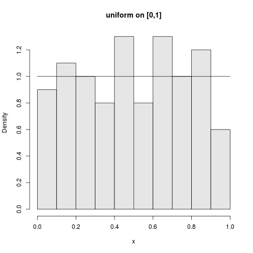
Fig. Histogram of uniform distribution
Normal distribution
function: rnorm()
arguments:
- n = sample size
- mean = mean of sample
- sd = standard deviation of sample
Normal numbers are the backbone of classical statistical theory due to the central limit theorem The normal distribution has two parameters a mean and a standard deviation. These are the location and spread parameters. For example, IQs may be normally distributed with mean 100 and standard deviation 16; Human gestation may be normal with mean 280 and standard deviation of 10 (approximately). The family of normals can be standardized to normal with mean 0 (centered) and variance 1. This is achieved by "standardizing" the numbers, i.e. .
For example
# an IQ score
rnorm(n = 1, mean = 100, sd = 16)
## [1] 88.46
# gestation
rnorm(n = 1, mean = 280, sd = 10)
## [1] 279.6Too see the shape for the defaults (mean 0, standard deviation 1).
x = rnorm(n = 100)
hist(x, probability = TRUE, col = gray(0.9), main = "normal mu=0,sigma=1")
curve(dnorm(x), add = TRUE)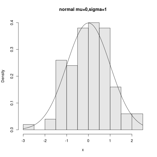
Fig. Histogram of normal distribution
Binomial.
function: rbinom()
arguments:
- n = number of observations
- size = number of trials
- prob = probability of success
The binomial random numbers are discrete random numbers. They have the distribution of the number of successes in n independent Bernoulli trials where a Bernoulli trial results in success or failure, with the probability of success = p
A single Bernoulli trial (e.g. a coin flip) is given with size = 1.
rbinom(n = 1, size = 1, prob = 0.5)## [1] 0
# 10 different numbers
rbinom(n = 10, size = 1, prob = 0.5)
## [1] 0 0 1 1 1 0 1 0 0 0A binomially distributed number is the same as the number of 1's in n such Bernoulli numbers.
To generate binomial numbers, we simply change the value of size from 1 to the desired number of trials. For example, with 10 trials:
# how many successes in 10 trials
rbinom(n = 1, size = 10, p = 0.5)
## [1] 5
# 5 separate series of 10 trials
rbinom(n = 5, size = 10, p = 0.5)
## [1] 4 5 4 5 6The number of successes is of course discrete, but as n gets large, the number starts to look quite normal. This is a case of the central limit theorem which states in general that is normal in the limit.
These graphs show 100 binomially distributed random numbers for size = 5 trials and for p = 0.25.
# 100 random numbers
x = rbinom(100, size = 5, p = 0.25)
hist(x, probability = TRUE)

# use points, not curve as dbinom() wants integers only for x
xvals = 0:5
points(xvals, dbinom(xvals, 5, 0.25), type = "h", lwd = 3)
points(xvals, dbinom(xvals, 5, 0.25), type = "p", lwd = 3)
Fig. Histograms of binomial distributions
Exponential
function: rexp()
arguments:
- n = sample size
- rate = (vector of) rate of exponential decay
The exponential distribution is important for theoretical work. It is used to describe lifetimes of electrical components (to first order). For example, if the mean life of a light bulb is 2500 hours one may think its lifetime is random with exponential distribution having mean 2500. The one parameter is the . We specify it as follows
rexp(n, rate = 1).
Here is an example with the rate being 1/2500.
x = rexp(n = 100, rate = 1/2500)
hist(x, probability = TRUE, col = gray(0.9), main = "exponential mean=2500")
curve(dexp(x, 1/2500), add = TRUE)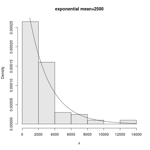
Fig. Histogram of exponential distribution
There are many other distributions of interest in statistics. Common ones are the Poisson, the Student t-distribution, the F distribution, the beta distribution and the Chi squared distribution. All are available in R and follow similar format to these outlined above.
Random Sampling / Bootstrapping
We can use the sample() function to randomly pull values, with or without replacement, from a vector. b is the vector that you want to sample from, size is the number of times to randomly pull a value from b.
b <- 1:6
sample(b, size = 10, replace = TRUE)
## [1] 2 5 2 5 2 4 4 1 3 6
# or with a function
RollDie = function(n) sample(1:6, n, replace = TRUE)

# Roll five dice three times...
RollDie(5)
## [1] 5 6 1 4 3RollDie(5)## [1] 5 2 4 2 2RollDie(5)## [1] 3 4 5 6 6Sampling with and without replacement using sample()
R has the ability to sample with and without replacement. That is, choose at random from a collection of things such as the numbers 1 through 6 in the dice rolling example.
The sampling can be done with replacement (like dice rolling) or without replacement (like a lottery). By default sample() samples without replacement each object having equal chance of being picked. You need to specify replace = TRUE if you want to sample with replacement. Furthermore, you can specify separate probabilities for each if desired.
Roll a die ten times
sample(1:6, 10, replace = TRUE)## [1] 1 2 6 4 1 3 2 3 5 2Toss a coin
sample(c("H", "T"), 10, replace = TRUE)## [1] "T" "T" "T" "H" "H" "T" "H" "T" "T" "T"Pick 6 of 54 (a lottery)
sample(1:54, 6) # no replacement## [1] 47 25 18 13 22 36Pick a card. (Fancy! Uses paste, rep)
cards <- paste(rep(c("A", 2:10, "J", "Q", "K"), 4), c("H", "D", "S", "C"))
sample(cards, 5)
## [1] "J D" "8 D" "8 H" "3 C" "J H"Roll 2 dice. Even fancier
dice <- as.vector(outer(1:6, 1:6, paste))
sample(dice, 5, replace = TRUE)
## [1] "5 4" "2 1" "3 2" "5 6" "6 6"The last two illustrate things that can be done with a little typing and a lot of thinking using the fun commands paste() for pasting together strings, rep() for repeating things and outer() for generating all possible products.
A bootstrap sample
Bootstrapping is a method of sampling from a data set to make statistical inference. The intuitive idea is that by sampling, one can get an idea of the variability in the data. The process involves repeatedly selecting samples and then forming a statistic. Here is a simple illustration on obtaining a sample.
The built-in data set faithful has a variable "eruptions" that measures the time between eruptions at Old Faithful. It has an unusual distribution. A bootstrap sample is just a sample with replacement from the given values.
First, examine the dataset
data(faithful)  # part of R's base
names(faithful)
## [1] "eruptions" "waiting"head(faithful)## eruptions waiting
## 1 3.600 79
## 2 1.800 54
## 3 3.333 74
## 4 2.283 62
## 5 4.533 85
## 6 2.883 55
eruptions <- faithful$eruptions
sample(eruptions, 10, replace = TRUE)  # a sample of 10 values
## [1] 2.800 4.350 4.133 1.867 4.533 2.017 2.133 2.617 4.233 4.250
# Plot the full dataset
hist(eruptions, breaks = 25)
plot of chunk unnamed-chunk-11
Second, obtain the bootstrap sample
hist(sample(eruptions, 100, replace = TRUE), breaks = 25)
Fig. Histogram of eruptions.
Notice that the bootstrap sample has a similar histogram, but it is different:
par(mfrow = c(2, 1))
hist(eruptions, breaks = 25)
hist(sample(eruptions, 100, replace = TRUE), breaks = 25)
Fig. Histogram of (top) eruptions, and (bottomw) bootstrapped sample.