Testing Assumptions

Functions: fitted(), residuals(), acf(), bartlett.test(), filger.test(), qqline(), shapiro.test(), ks.test()

Code: .r .txt

All statistical tests have assumptions. The validity of any conclusion drawn from a statistical test depends in large part on the validity of the assumptions made.

These assumptions come under three broad categories:

Distributional assumptions are concerned with the probability distributions of the observations or their associated random errors (e.g., normal versus binomial).
Structural assumptions are concerned with the form of the functional relationships between the response variable and the predictor variables (e.g., linear regression assumes that the relationsip is linear).
Cross-variation assumptions are concerned with the joint probability distribution of the observations and/or the errors (e.g., most tests assume that the observations are independent).

We emphasize the visual inspection of the data and model, rather than an over-reliance on statistical tests of the assumptions.

Linear Regression and ANOVA

Linear regression and ANOVA have four assumptions.

We will examine them using the large sparrow data.

dat <- read.table(file = "http://www.simonqueenborough.info/R/data/sparrows.txt", header = TRUE)
head(dat)

##   Species    Sex Wingcrd Tarsus Head Culmen Nalospi   Wt Observer Age
## 1    SSTS   Male    58.0   21.7 32.7   13.9    10.2 20.3        2   0
## 2    SSTS Female    56.5   21.1 31.4   12.2    10.1 17.4        2   0
## 3    SSTS   Male    59.0   21.0 33.3   13.8    10.0 21.0        2   0
## 4    SSTS   Male    59.0   21.3 32.5   13.2     9.9 21.0        2   0
## 5    SSTS   Male    57.0   21.0 32.5   13.8     9.9 19.8        2   0
## 6    SSTS Female    57.0   20.7 32.5   13.3     9.9 17.5        2   0

m <- lm(Head ~ Sex + Tarsus, data = dat)

We will need to look at the residuals and predicted/fitted values from the model, as well as the original data.

We can extract the values from the model in two ways.

Either directly from the model itself:

m$residuals
m$fitted

Or, via functions:

fitted(m)
residuals(m)

1. Linearity and additivity of the relationship between dependent and independent variables:

Violation is serious and likely leads to errors in prediction especially when extrapolating beyond the data.

Diagnosis:

i. Plot of observed versus predicted values.

The points should be symmetrically distributed around a diagonal line, with a roughly constant variance.

# Here, the observed (dat$Head) on predicted (or fitted: m$fitted.values)
plot(dat$Head ~ m$fitted.values)

# add 1:1 line
abline(0, 1)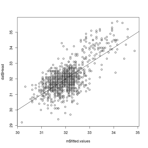

plot of chunk obs-v-fitted

ii. Plot of residuals versus predicted values.

The points should be symmetrically distributed around a horizontal line, with a roughly constant variance.

# Here, the residuals (m$residuals) on predicted (or fitted: m$fitted.values)
plot(m$residual ~ m$fitted.values)

# add horizontal line at 0
abline(h = 0)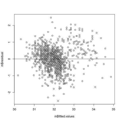

plot of chunk resid-v-fitted

iii. Plots of the residuals versus individual independent variables.

par(mfrow = c(1,2))
plot(m$residual ~ dat$Tarsus)
plot(m$residual ~ dat$Sex)

plot of chunk resid-v-data

2. Statistical independence of the errors (in particular, no correlation between consecutive errors in the case of time series data)

This assumption is particularly important for data that are known to be autocorrelated (time series, spatial data). However, it is possible that the predictor variables account for the autocorrelation.

Diagnosis

i. Plot of residuals versus time series/row number.

plot(m$resid)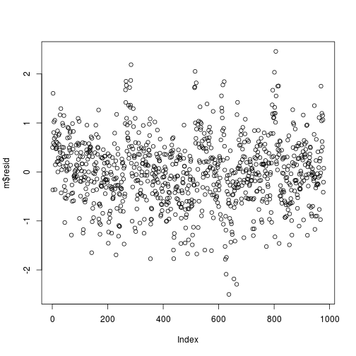

plot of chunk resid-row

ii. Plot estimates of the autocorrelation function

The X axis corresponds to the lags of the residual, increasing in steps of 1. The very first line (to the left) shows the correlation of residual with itself (Lag0), therefore, it will always be equal to 1.

If the residuals were not autocorrelated, the correlation (Y-axis) from the immediate next line onwards will drop to a near zero value below the dashed blue line (significance level).

acf(m$resid)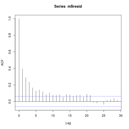

plot of chunk resid-acf

iii. Plot of residuals versus Moran's I.

For tests of spatial autocorrelation, see this page:

http://www.ats.ucla.edu/stat/mult_pkg/faq/general/spatial_autocorr.htm

3. Homoscedasticity (constant variance) of the errors

Violations of constant variance make it hard to estimate the standard deviation of the coefficient estimates.

Diagnosis

Check for consistent change in the residuals in the following plots.

i. Plot residuals versus time (in the case of time series data).

ii. Plots residuals versus the predicted values.

# Here, the residuals (m$residuals) on predicted (or fitted: m$fitted.values)
plot(m$residual ~ m$fitted.values)

# add horizontal line at 0
abline(h = 0)

plot of chunk resid-v-fitted2

iii. Plot residuals versus independent variables.

par(mfrow = c(1,2))
plot(m$residual ~ dat$Tarsus)
plot(m$residual ~ dat$Sex)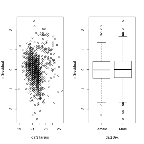

plot of chunk resid-v-data2

The bartlett.test() function provides a parametric K-sample test of the equality of variances.

bartlett.test(m$residual ~ dat$Sex)

## 
##  Bartlett test of homogeneity of variances
## 
## data:  m$residual by dat$Sex
## Bartlett's K-squared = 0.013474, df = 1, p-value = 0.9076

The `fligner.test()``` function provides a non-parametric test of the same.

fligner.test(m$residual ~ dat$Sex)

## 
##  Fligner-Killeen test of homogeneity of variances
## 
## data:  m$residual by dat$Sex
## Fligner-Killeen:med chi-squared = 0.023968, df = 1, p-value =
## 0.877

3. Normality of the error distribution.

Violations of normality create problems for determining whether model coefficients are significantly different from zero and for calculating confidence intervals. It is not required for estimating the coefficients.

Outliers Parameter estimation is based on the minimization of squared error, thus a few extreme observations can exert a disproportionate influence on parameter estimates.

Diagnosis

The histogram of the residuals looks ok ...

hist(m$resid)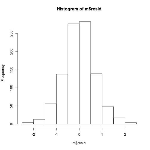

plot of chunk resid-hist

i. Normal probability plot or normal quantile plot of the residuals.

These are plots of the fractiles of error distribution versus the fractiles of a normal distribution with the same mean and variance.

qqnorm(m$resid)
qqline(m$resid)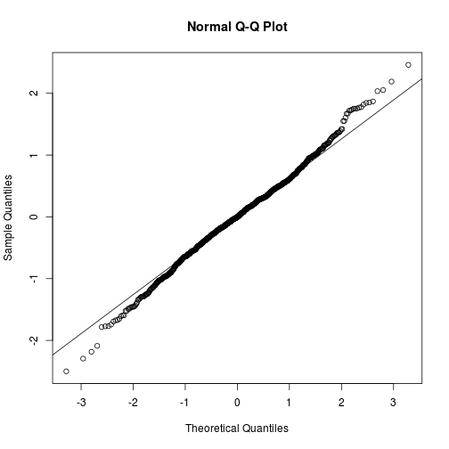

plot of chunk resid-qq

A normal distribution is indicated by the points lying close to the diagonal reference line.

A bow-shaped pattern of deviations from the diagonal indicates that the residuals have excessive skewness (i.e., they are not symmetrically distributed, with too many large errors in one direction).

An S-shaped pattern of deviations indicates that the residuals have excessive kurtosis (i.e., there are either too many or two few large errors in both directions).

ii.Outliers

Outliers are indicated by data points on one or both ends that deviate significantly from the reference line.

stripchart(dat$Head~dat$Sex, vertical = TRUE, method = 'jitter', col = c('darkgrey', 'red'), pch = 21)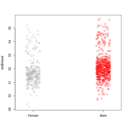

plot of chunk head-v-sex

ii. Statistical tests for normality

These two tests are available in base R

Kolmogorov-Smirnov test

ks.test(m$resid, pnorm)

## Warning in ks.test(m$resid, pnorm): ties should not be present for the
## Kolmogorov-Smirnov test

## 
##  One-sample Kolmogorov-Smirnov test
## 
## data:  m$resid
## D = 0.11356, p-value = 2.159e-11
## alternative hypothesis: two-sided

Shapiro-Wilk test

shapiro.test(m$resid)

## 
##  Shapiro-Wilk normality test
## 
## data:  m$resid
## W = 0.99525, p-value = 0.003809

# This distribution is not normal

Other tests, such as the Jarque-Bera test, Anderson-Darling test, are available in other packages. This page has a good discussion of such tests https://stats.stackexchange.com/questions/90697/is-shapiro-wilk-the-best-normality-test-why-might-it-be-better-than-other-tests?noredirect=1&lq=1

However, real data with perfect normal errors are extremely rare.

Using plot()

Using the function plot() on a model will generate four figures that test many of the above assumptions.

par(mfrow = c(2,2))
plot(m)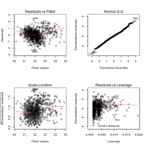

plot of chunk plot-test

Top-left: Residuals versus fitted values. Testing for linearity and constant variance of residuals.

Top-right: Q-q plot. Testing for normality of residuals.

Bottom-left: Square root residuals versus fitted values. Testing for linearity and constant variance of residuals.

Bottom-right: Standardized residuals versus leverage. Leverage is a measure of how much each data point influences the regression. The plot also adds values of Cook's distance, which reflects how much the fitted values would change if a point was deleted. For a good regression model, the red smoothed line should stay close to the mid-line and no point should have a large Cook’s distance (i.e. should not have too much influence on the model.)

Exercises

Test the assumptions of the model above for male and female sparrows separately.

Do different continuous predictors of response variables better fit the assumptions?

Updated: 2016-11-14