Is There An Association Between Two (or More) Variables?
Functions: ks.test, cor, cor.test, lm
Categorical Variables
We use a Chi-Squared test of association for the different levels of two categorical variables.
See Testing Ratios for more details.
Two Continuous Variables
Do these samples come from the same distribution? Kolmogorov-Smirnov Test: ks.test()
# Generate 50 values drawn randomly from two different distributions: x is from a normal distribution and y from a uniform.
# Thus, we *know* they should be different
x <- rnorm(50)
y <- runif(30)

# Do x and y come from the same distribution?
ks.test(x, y)
##
## Two-sample Kolmogorov-Smirnov test
##
## data: x and y
## D = 0.53333, p-value = 2.159e-05
## alternative hypothesis: two-sidedThe p < 0.001 suggests that x and y are indeed drawn from different distributions.
Correlation: cor.test()
Let's look at the small sparrow dataset, and the relationship between the various measurements.
BirdData <- data.frame(
            Tarsus  = c(22.3, 19.7, 20.8, 20.3, 20.8, 21.5, 20.6, 21.5),
            Head    = c(31.2, 30.4, 30.6, 30.3, 30.3, 30.8, 32.5, 31.6),
            Weight  = c(9.5, 13.8, 14.8, 15.2, 15.5, 15.6, 15.6, 15.7),
            Wingcrd = c(59, 55, 53.5, 55, 52.5, 57.5, 53, 55),
            Species = c('A', 'A', 'A', 'A', 'A',  'B', 'B', 'B')
            )
Then, make a 2x2 panel plot.
par(mfrow = c(2, 2))
plot(BirdData$Tarsus ~ BirdData$Wingcrd)
plot(BirdData$Tarsus ~ BirdData$Head)
plot(BirdData$Tarsus ~ BirdData$Weight)
plot(BirdData$Head ~ BirdData$Wingcrd)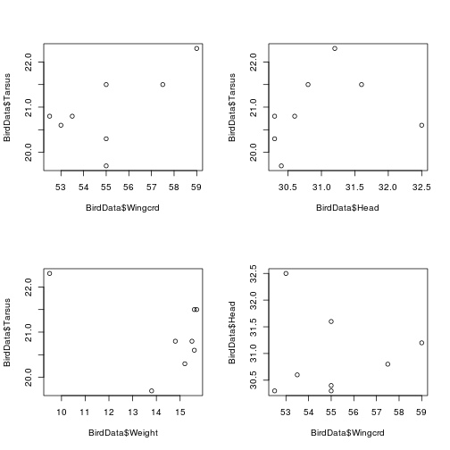
Fig. The relationships between measurements of sparrows
We have no a priori reason to believe that any of these measurements of sparrows drives variation in the others. However, we can test whether they are correlated. For example, do sparrows with larger heads also have larger wings?
The function cor() returns the correlation coefficient of two variables. It requires an x and a y. Pearson's product moment correlation coefficient is the parametric version used for normal data; Kendall's tau or Spearman's rho for non-parametric data.
cor(x = BirdData$Tarsus, y = BirdData$Wingcrd, method = 'pearson')## [1] 0.6409484The function cor.test() tests for association---correlation---between paired samples, using one of Pearson's product moment correlation coefficient, Kendall's tau or Spearman's rho, as above. The three methods each estimate the association between paired samples and compute a test of the value being zero (indicating no association). We use the method = argument to specify which (Pearson is the default).
Pearson should be used if the samples follow independent normal distributions. Kendall's tau or Spearman's rho statistic is used to estimate a rank-based measure of association. These tests may be used if the data do not necessarily come from a bivariate normal distribution.
cor.test(x = BirdData$Tarsus, y = BirdData$Wingcrd, method = 'pearson')##
## Pearson's product-moment correlation
##
## data: BirdData$Tarsus and BirdData$Wingcrd
## t = 2.0454, df = 6, p-value = 0.0868
## alternative hypothesis: true correlation is not equal to 0
## 95 percent confidence interval:
## -0.1162134 0.9269541
## sample estimates:
## cor
## 0.6409484Because it is a test of correlation, with no causality, if we want to use the formula = argument, we have to set it up slightly differently.
cor.test(formula = ~ BirdData$Tarsus + BirdData$Wingcrd)##
## Pearson's product-moment correlation
##
## data: BirdData$Tarsus and BirdData$Wingcrd
## t = 2.0454, df = 6, p-value = 0.0868
## alternative hypothesis: true correlation is not equal to 0
## 95 percent confidence interval:
## -0.1162134 0.9269541
## sample estimates:
## cor
## 0.6409484Simple Linear Regression: lm()
If we think that one variable is driving variation in the other, we should use regression rather than correlation.
The function lm() is used to develop linear models. At its simplest, it takes one argument: formula
Models are specified symbolically. A typical model has the form response ~ terms where response is the (numeric) response/dependent vector and terms is a series of terms which specifies a linear predictor (or independent variable) for response.
The response variable is fitted as a function of the predictor variable. The tilde symbol (~) signifies as a function of, and separates the response and predictor variables. Adding further predictor variables to the right hand side is possible (see Formulae).
For now, we will carry out a simple regression of a single predictor and response. This model estimates values for the three elements of the equation:
y ~ beta0 + beta1 * x + sigma
In other words:
y ~ intercept + slope * x + sd of the error
We will come back to this later.
We will illustrate the use of lm() using the sparrow data (even though we know there is no causality here).
First, we plot the data.
plot(BirdData$Tarsus ~ BirdData$Wingcrd)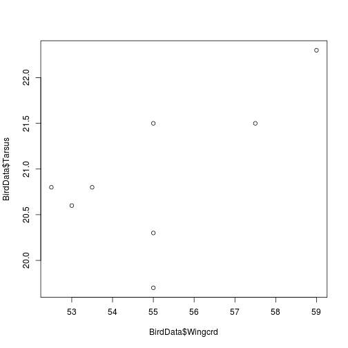
Fig. Sparrow Wingcrd as a function of Tarsus length
Second, we run the model.
m <- lm(BirdData$Tarsus ~ BirdData$Wingcrd)

# or
m <- lm(Tarsus ~ Wingcrd, data = BirdData)
Examining the output
The output of lm() is a list. We can use str() to examine the elements of the output, as well as pull out various parts directly, or use other functions to do so.
For example, summary() returns the whole model table,
summary(m)##
## Call:
## lm(formula = Tarsus ~ Wingcrd, data = BirdData)
##
## Residuals:
## Min 1Q Median 3Q Max
## -1.2229 -0.1594 0.1844 0.4492 0.5770
##
## Coefficients:
## Estimate Std. Error t value Pr(>|t|)
## (Intercept) 8.1210 6.2706 1.295 0.2429
## Wingcrd 0.2328 0.1138 2.045 0.0868 .
## ---
## Signif. codes: 0 '***' 0.001 '**' 0.01 '*' 0.05 '.' 0.1 ' ' 1
##
## Residual standard error: 0.6705 on 6 degrees of freedom
## Multiple R-squared: 0.4108, Adjusted R-squared: 0.3126
## F-statistic: 4.184 on 1 and 6 DF, p-value: 0.0868coef() the coefficients,
coef(m)## (Intercept) Wingcrd
## 8.1209721 0.2327633and resid() returns the residuals.
resid(m)## 1 2 3 4 5
## 0.445994599 -1.222952295 0.226192619 -0.622952295 0.458955896
## 6 7 8
## -0.004860486 0.142574257 0.577047705Adding a fitted line to a plot
we can use abline() to add the fitted line of the model to a plot of the raw data.
plot(BirdData$Tarsus ~ BirdData$Wingcrd)
abline(lm(BirdData$Tarsus ~ BirdData$Wingcrd))

# or
m <- lm(BirdData$Tarsus ~ BirdData$Wingcrd)
abline(m)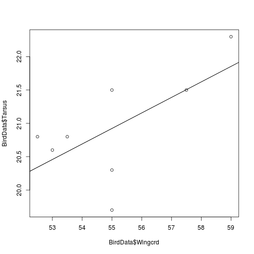
Fig. Sparrow Wingcrd as a function of Tarsus length, with fitted line
Exercises
Using the New Haven Road Race data, test for a correlation between the Pace and Net time.
Using the large sparrow data set, test for correlations between the 5 continous variables. Plot the data and add fitted lines.
Updated: 2016-10-27