Spatial point patterns
CRAN spatial page
The most comprehensive package for spatial point pattern analysis is Spatstat, which also has a more detailed course on spatial stats
library(spatstat)## Loading required package: mgcv
## Loading required package: nlme
## This is mgcv 1.7-27. For overview type 'help("mgcv-package")'.
## Loading required package: deldir
## deldir 0.1-1
##
## spatstat 1.33-0 (nickname: 'Titanic Deckchair')
## For an introduction to spatstat, type 'beginner'Run this to see some examples of the kind of data spatstat works with
demo(data)Overview
data(swedishpines)
plot(swedishpines)
swedishpines## planar point pattern: 71 points
## window: rectangle = [0, 96] x [0, 100] units (one unit = 0.1 metres)
summary(swedishpines)## Planar point pattern: 71 points
## Average intensity 0.0074 points per square unit (one unit = 0.1 metres)
##
## Coordinates are integers
## i.e. rounded to the nearest 1 unit (one unit = 0.1 metres)
##
## Window: rectangle = [0, 96] x [0, 100] units
## Window area = 9600 square units
## Unit of length: 0.1 metresdensity plot
plot(density(swedishpines, 10))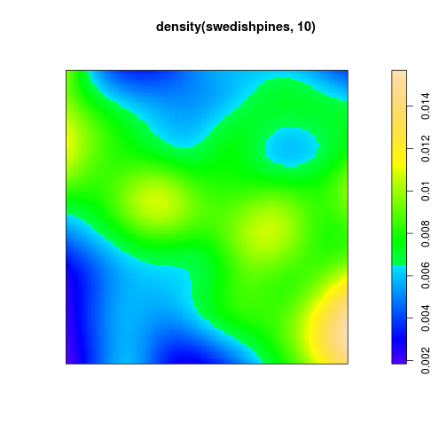
plot of chunk densplot
contour plot
contour(density(swedishpines, 10), axes = FALSE)
quadrat counting
Q <- quadratcount(swedishpines, nx = 4, ny = 3)
Q
## x
## y [0,24] (24,48] (48,72] (72,96]
## (66.7,100] 7 3 6 5
## (33.3,66.7] 5 9 7 7
## [0,33.3] 4 3 6 9
plot(swedishpines)
plot(Q, add = TRUE, cex = 2)
point pattern analysis: the K function
par(mfrow = c(1, 2))
K <- Kest(swedishpines)
plot(K)
## lty col key label
## iso 1 1 iso hat(K)[iso](r)
## trans 2 2 trans hat(K)[trans](r)
## border 3 3 border hat(K)[bord](r)
## theo 4 4 theo K[pois](r)
## meaning
## iso Ripley isotropic correction estimate of K(r)
## trans translation-corrected estimate of K(r)
## border border-corrected estimate of K(r)
## theo theoretical Poisson K(r)
E <- envelope(Y = swedishpines, fun = Kest, nsim = 39)## Generating 39 simulations of CSR ...
## 1, 2, 3, 4, 5, 6, 7, 8, 9, 10, 11, 12, 13, 14, 15,
## 16, 17, 18, 19, 20, 21, 22, 23, 24, 25, 26, 27, 28, 29, 30,
## 31, 32, 33, 34, 35, 36, 37, 38, 39.
##
## Done.plot(E)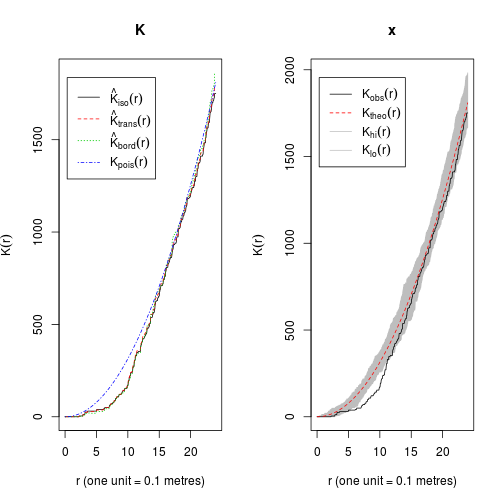
## lty col key label
## obs 1 1 obs K[obs](r)
## theo 2 2 theo K[theo](r)
## hi 1 8 hi K[hi](r)
## lo 1 8 lo K[lo](r)
## meaning
## obs observed value of K(r) for data pattern
## theo theoretical value of K(r) for CSR
## hi upper pointwise envelope of K(r) from simulations
## lo lower pointwise envelope of K(r) from simulationsModels
data(swedishpines)
X <- swedishpines
fit <- ppm(Q = X, trend = ~1, Strauss(9))
fit## Stationary Strauss process
##
## First order term:
## beta
## 0.05458
##
## Interaction: Strauss process
## interaction distance: 9
## Fitted interaction parameter gamma: 0.2645
##
## Relevant coefficients:
## Interaction
## -1.33
##
## For standard errors, type coef(summary(x))
# plot model:
plot(simulate(fit))
# goodness of fit test for model:
plot(envelope(Y = fit, fun = Kest, nsim = 39)) # good agreement!## Generating 39 simulated realisations of fitted Gibbs model ...
## 1, 2, 3, 4, 5, 6, 7, 8, 9, 10, 11, 12, 13, 14, 15,
## 16, 17, 18, 19, 20, 21, 22, 23, 24, 25, 26, 27, 28, 29, 30,
## 31, 32, 33, 34, 35, 36, 37, 38, 39.
##
## Done.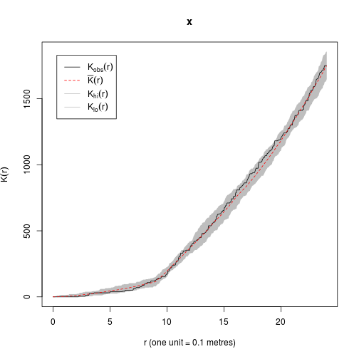
## lty col key label
## obs 1 1 obs K[obs](r)
## mmean 2 2 mmean bar(K)(r)
## hi 1 8 hi K[hi](r)
## lo 1 8 lo K[lo](r)
## meaning
## obs observed value of K(r) for data pattern
## mmean sample mean of K(r) from simulations
## hi upper pointwise envelope of K(r) from simulations
## lo lower pointwise envelope of K(r) from simulationsmultitype point patterns
data(lansing)
lansing## marked planar point pattern: 2251 points
## multitype, with levels = blackoak hickory maple misc redoak whiteoak
## window: rectangle = [0, 1] x [0, 1] units (one unit = 924 feet)
summary(lansing)## Marked planar point pattern: 2251 points
## Average intensity 2250 points per square unit (one unit = 924 feet)
##
## *Pattern contains duplicated points*
##
## Coordinates are given to 3 decimal places
## i.e. rounded to the nearest multiple of 0.001 units (one unit = 924 feet)
##
## Multitype:
## frequency proportion intensity
## blackoak 135 0.0600 135
## hickory 703 0.3120 703
## maple 514 0.2280 514
## misc 105 0.0466 105
## redoak 346 0.1540 346
## whiteoak 448 0.1990 448
##
## Window: rectangle = [0, 1] x [0, 1] units
## Window area = 1 square unit
## Unit of length: 924 feetplot(lansing)
## blackoak hickory maple misc redoak whiteoak
## 1 2 3 4 5 6plot(split(lansing))
hick <- split(lansing)$hickory
plot(hick)
Entering data
We can generate some random coordinates using the rnorm() function
x <- rnorm(10)
y <- rnorm(10)
plot(x, y)
And convert them to spatstat format as follows
dat <- ppp(x = x, y = y, xrange = c(-2, 2), yrange = c(-2, 2))## Warning: 3 points were rejected as lying outside the specified windowplot(dat)## Warning: 3 illegal points also plotted
Marks
A mark is an additional attribute of each point, e.g. height, species, ...
# first generate a sequence of two species marks
Sp <- c(rep("A", 5), rep("B", 5))
# include this vector in the ```ppp()``` call
dat <- ppp(x = x, y = y, xrange = c(-2, 2), yrange = c(-2, 2), marks = Sp)## Warning: 3 points were rejected as lying outside the specified windowWe can also assign a variety of marks to each point, using a dataframe
DBH <- round(rpois(10, 3) + rnorm(10), 2)
M <- data.frame(Sp = Sp, DBH = DBH)
M## Sp DBH
## 1 A 4.06
## 2 A 3.96
## 3 A 4.76
## 4 A 1.68
## 5 A 4.14
## 6 B 1.87
## 7 B 4.71
## 8 B 1.38
## 9 B 3.42
## 10 B -0.40
dat <- ppp(x = x, y = y, xrange = c(-2, 2), yrange = c(-2, 2), marks = M)## Warning: 3 points were rejected as lying outside the specified windowWe can plot these
par(mfrow = c(1, 2))
plot(dat)
plot(dat, which.marks = "DBH")## Plotting the first column of marks## Warning: Some marks are NA; corresponding points are omitted.
## Warning: 3 illegal points also plotted
## 1 1.5 2 2.5 3 3.5 4 4.5 5
## 0.08407 0.12611 0.16814 0.21018 0.25222 0.29425 0.33629 0.37832 0.42036Intensity
uniform/homogeneous intensity
data(swedishpines)
summary(swedishpines)## Planar point pattern: 71 points
## Average intensity 0.0074 points per square unit (one unit = 0.1 metres)
##
## Coordinates are integers
## i.e. rounded to the nearest 1 unit (one unit = 0.1 metres)
##
## Window: rectangle = [0, 96] x [0, 100] units
## Window area = 9600 square units
## Unit of length: 0.1 metres
summary(swedishpines)$intensity## [1] 0.007396inhomogeneous intensity
data(bei)
quadratcount(bei, nx = 4, ny = 2)## x
## y [0,250] (250,500] (500,750] (750,1e+03]
## (250,500] 666 677 130 481
## [0,250] 544 165 643 298Q <- quadratcount(bei, nx = 6, ny = 3)
plot(bei, cex = 0.5, pch = "+")
plot(Q, add = TRUE, cex = 2)
spatial covariates
slope <- bei.extra$grad
par(mfrow = c(1, 2))
plot(bei)
plot(slope)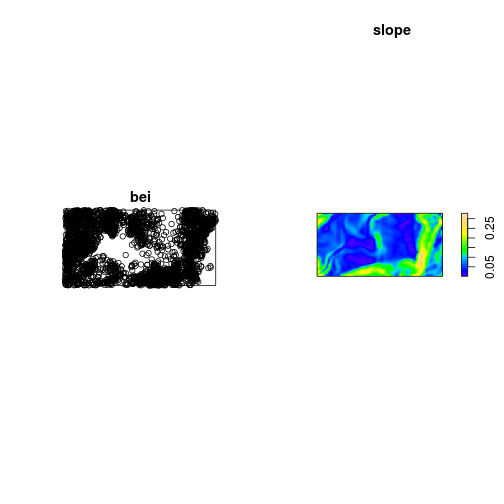
Z <- bei.extra$grad
b <- quantile(Z, probs = (0:4)/4)
Zcut <- cut(Z, breaks = b, labels = 1:4) # divide plot area up into 4 different slope types
V <- tess(image = Zcut)
plot(V)## Interpreting pixel values as coloursplot(bei, add = TRUE, pch = "+")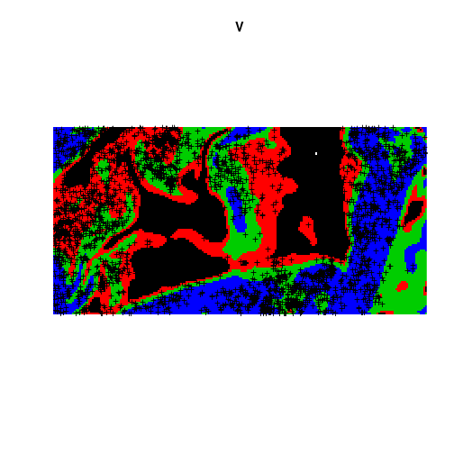
quadratcount(bei, tess = V)## tile
## 1 2 3 4
## 271 984 1028 1321Testing for Complete Spatial Randomness (CSR)
We can use quadrat counting, but there are problems with loss of data (pooled to quadrats), spatial scale and independence of data.
quadrat.test(bei, tess = V)##
## Chi-squared test of CSR using quadrat counts
##
## data: bei
## X-squared = 661.8, df = 3, p-value < 2.2e-16
## alternative hypothesis: two.sided
##
## Quadrats: 4 tiles (levels of a pixel image)A more powerful test is the kolmogorov-smirnov test, but only for continuous covariates.
KS <- kstest(bei, Z)
plot(KS)
KS##
## Spatial Kolmogorov-Smirnov test of CSR in two dimensions
##
## data: covariate 'Z' evaluated at points of 'bei'
## and transformed to uniform distribution under CSR
## D = 0.1948, p-value < 2.2e-16
## alternative hypothesis: two-sidedModels
Further methods for modelling spatial covariates are included in the Spatstat handbook.
Interactions
Points can be clustered (points tend to be close together), over-dispersed (points tend to avoid each other) or random (ie independent, Poisson).
The K function: kest()
The K function is the expected number of other points within a distance r of a typical point.
data(cells)
plot(Kest(cells))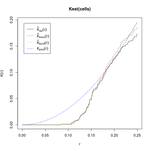
##        lty col    key            label
## iso      1   1    iso   hat(K)[iso](r)
## trans    2   2  trans hat(K)[trans](r)
## border   3   3 border  hat(K)[bord](r)
## theo     4   4   theo       K[pois](r)
##                                             meaning
## iso    Ripley isotropic correction estimate of K(r)
## trans        translation-corrected estimate of K(r)
## border            border-corrected estimate of K(r)
## theo theoretical Poisson K(r)L is common linear transformation of K, aiding interpretation.
- observed lines below theoretical line = over-dispersion
- observed lines above theoretical line = aggregation
L <- Lest(cells)
plot(L, main = "L function")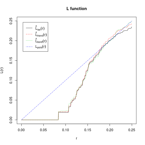
## lty col key label
## iso 1 1 iso hat(L)[iso](r)
## trans 2 2 trans hat(L)[trans](r)
## border 3 3 border hat(L)[bord](r)
## theo 4 4 theo L[pois](r)
## meaning
## iso Ripley isotropic correction estimate of L(r)
## trans translation-corrected estimate of L(r)
## border border-corrected estimate of L(r)
## theo theoretical Poisson L(r)We can use the envelope() function to calculate 'confidence limits' to the observed data.
E <- envelope(cells, Kest, nsim = 39, rank = 1)## Generating 39 simulations of CSR ...
## 1, 2, 3, 4, 5, 6, 7, 8, 9, 10, 11, 12, 13, 14, 15,
## 16, 17, 18, 19, 20, 21, 22, 23, 24, 25, 26, 27, 28, 29, 30,
## 31, 32, 33, 34, 35, 36, 37, 38, 39.
##
## Done.plot(E)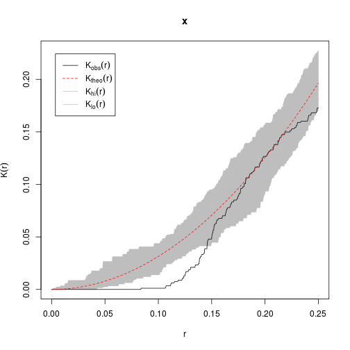
##      lty col  key      label
## obs    1   1  obs  K[obs](r)
## theo   2   2 theo K[theo](r)
## hi     1   8   hi   K[hi](r)
## lo     1   8   lo   K[lo](r)
##                                                meaning
## obs            observed value of K(r) for data pattern
## theo                 theoretical value of K(r) for CSR
## hi   upper pointwise envelope of K(r) from simulations
## lo lower pointwise envelope of K(r) from simulationsThese methods can be extended to a variety of models and spatial point processes, marked point patterns etc.