Very Brief Intro to Phylogenetic Comparative Methods in R

Good basic intro found here, which goes into more detail than presented here.

1. Tips vs PICS vs PGLS analyses

2. A) PICs in the 'ape' package

We use the package 'ape'

library(ape)

Load the tree and data for Geospiza sparrows

geodata <- read.table("../data/geospiza.txt")
geotree <- read.nexus("../data/geospiza.nex")

plot(wingL ~ tarsusL, geodata)

Drop tips for which no data

geotree <- drop.tip(geotree, "olivacea")

Create numeric vector for traits

wingL <- geodata$wingL
tarsusL <- geodata$tarsusL

Add rownames to allow R to associate data with correct names on tree

names(wingL) <- row.names(geodata)
names(tarsusL) <- row.names(geodata)

To calculate contrasts that have been scaled using the expected variances

ContrastwingL <- pic(wingL, geotree)
ContrasttarsusL <- pic(tarsusL, geotree)

Plot these

plot(geotree)
nodelabels(round(ContrastwingL, 3), adj = c(0, -0.5), frame = "n")
nodelabels(round(ContrasttarsusL, 3), adj = c(0, 1), frame = "n")

2. B) Correlated trait evolution

RegressTarsusWing <- lm(ContrastwingL ~ ContrasttarsusL - 1)
summary.lm(RegressTarsusWing)

## 
## Call:
## lm(formula = ContrastwingL ~ ContrasttarsusL - 1)
## 
## Residuals:
##     Min      1Q  Median      3Q     Max 
## -0.1077 -0.0418 -0.0257  0.0775  0.2551 
## 
## Coefficients:
##                 Estimate Std. Error t value Pr(>|t|)    
## ContrasttarsusL    1.076      0.157    6.86  2.7e-05 ***
## ---
## Signif. codes:  0 '***' 0.001 '**' 0.01 '*' 0.05 '.' 0.1 ' ' 1
## 
## Residual standard error: 0.126 on 11 degrees of freedom
## Multiple R-squared:  0.81,   Adjusted R-squared:  0.793 
## F-statistic:   47 on 1 and 11 DF,  p-value: 2.74e-05

plot(ContrastwingL, ContrasttarsusL)
abline(RegressTarsusWing)

3. PGLS in the 'ape' package

library(nlme)

Read in tree

geotree <- read.nexus("../data/geospiza.nex")
geospiza13.tree <- drop.tip(geotree, "olivacea")
geodata <- read.table("../data/geospiza.txt", row.names = 1)

Create specific dataframe

wingL <- geodata$wingL
tarsusL <- geodata$tarsusL
DF.geospiza <- data.frame(wingL, tarsusL, row.names = row.names(geodata))
DF.geospiza <- DF.geospiza[geospiza13.tree$tip.label, ]
DF.geospiza

##              wingL tarsusL
## fuliginosa   4.133   2.807
## fortis       4.244   2.895
## magnirostris 4.404   3.039
## conirostris  4.350   2.984
## scandens     4.261   2.929
## difficilis   4.224   2.899
## pallida      4.265   3.089
## parvulus     4.132   2.973
## psittacula   4.235   3.049
## pauper       4.232   3.036
## Platyspiza   4.420   3.271
## fusca        3.975   2.937
## Pinaroloxias 4.189   2.980

Correlation structure

bm.geospiza <- corBrownian(phy = geospiza13.tree)

Model

bm.gls <- gls(wingL ~ tarsusL, correlation = bm.geospiza, data = DF.geospiza)
summary(bm.gls)

## Generalized least squares fit by REML
##   Model: wingL ~ tarsusL 
##   Data: DF.geospiza 
##      AIC    BIC logLik
##   -25.88 -24.69  15.94
## 
## Correlation Structure: corBrownian
##  Formula: ~1 
##  Parameter estimate(s):
## numeric(0)
## 
## Coefficients:
##              Value Std.Error t-value p-value
## (Intercept) 0.9547    0.4767   2.003  0.0705
## tarsusL     1.0764    0.1570   6.857  0.0000
## 
##  Correlation: 
##         (Intr)
## tarsusL -0.995
## 
## Standardized residuals:
##     Min      Q1     Med      Q3     Max 
## -1.4607 -0.1545  0.2701  1.6376  1.9047 
## 
## Residual standard error: 0.09603 
## Degrees of freedom: 13 total; 11 residual

4. PGLS in the 'caper' package

library(caper)

## Loading required package: MASS
## Loading required package: mvtnorm

Create new column of names

geodata$Names <- rownames(geodata)

Create comparative data object, combining the data and tree, and removing data/tips.

cdat <- comparative.data(data = geodata, phy = geotree, names.col = "Names")

Test correlation of wing and tarsus as before

m <- pgls(wingL ~ tarsusL, data = cdat, lambda = "ML")
summary(m)

## 
## Call:
## pgls(formula = wingL ~ tarsusL, data = cdat, lambda = "ML")
## 
## Residuals:
##     Min      1Q  Median      3Q     Max 
## -0.1486 -0.0208  0.0467  0.0596  0.3356 
## 
## Branch length transformations:
## 
## kappa  [Fix]  : 1.000
## lambda [ ML]  : 1.000
##    lower bound : 0.000, p = 0.00034
##    upper bound : 1.000, p = 1    
##    95.0% CI   : (0.837, NA)
## delta  [Fix]  : 1.000
## 
## Coefficients:
##             Estimate Std. Error t value Pr(>|t|)    
## (Intercept)    0.955      0.477    2.00     0.07 .  
## tarsusL        1.076      0.157    6.86  2.7e-05 ***
## ---
## Signif. codes:  0 '***' 0.001 '**' 0.01 '*' 0.05 '.' 0.1 ' ' 1
## 
## Residual standard error: 0.126 on 11 degrees of freedom
## Multiple R-squared: 0.81,    Adjusted R-squared: 0.793 
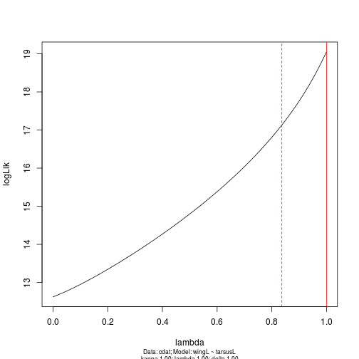
## F-statistic:   47 on 2 and 11 DF,  p-value: 4.08e-06

Estimate phylogenetic correlation and plot it (in this case, we have a strong phylogenetic signal in the data)

m.profile <- pgls.profile(m, "lambda")
plot(m.profile)

---