Meta-analysis

analysis of analyses

A meta-analysis is the synthesis of

It gives greater weight to studies with less variance and more precision.

NB: A meta-analysis starts with a systematic review.

Effects

An "effect" could be almost any aggregate statistic of interest:

Mean, Mean difference, Mean change
Risk ratio, Odds ratio, Risk difference
Incidence rate, Prevalence, Proportion
Correlation

Packages

meta (Author: Guido Schwarzer)
metafor (Author: Wolfgang Viechtbauer)
rmeta (Author: Thomas Lumley)

1. Calculate effect sizes

The escalc() function in the metafor package calculates effect sizes.

Provide necessary data components (sample size, events in each treatment group, etc.).
Indicate the effect size you want to measure.

ES <- escalc(endpoints, variances, measure, data, ...)

endpoints: arguments or formula containing endpoint values
variances: arguments containing endpoint variances
measure: character value indicating type of effect size
data: data frame containing named variables

The measure (type of effect size) will then influence what endpoint and variance inputs are needed.

See ?escalc for more details.

Example: BCG vaccine trials (from metafor)

Overview: 13 vaccine trials of Bacillus Calmette-Guerin (BCG) vaccine vs. no vaccine

Treatment goal: Prevention of tuberculosis

Primary endpoint: Tuberculosis infection

Possible explanatory variables:

latitude of study region ($ablat)
treatment allocation method ($alloc)
year published ($year)

library(metafor)  # Load package

## Loading required package: Matrix
## Loading 'metafor' package (version 1.9-8). For an overview 
## and introduction to the package please type: help(metafor).

data(dat.bcg)  # BCG meta-analytic dataset
str(dat.bcg)  # Describe meta-analysis structure

## 'data.frame':    13 obs. of  9 variables:
##  $ trial : int  1 2 3 4 5 6 7 8 9 10 ...
##  $ author: chr  "Aronson" "Ferguson & Simes" "Rosenthal et al" "Hart & Sutherland" ...
##  $ year  : int  1948 1949 1960 1977 1973 1953 1973 1980 1968 1961 ...
##  $ tpos  : int  4 6 3 62 33 180 8 505 29 17 ...
##  $ tneg  : int  119 300 228 13536 5036 1361 2537 87886 7470 1699 ...
##  $ cpos  : int  11 29 11 248 47 372 10 499 45 65 ...
##  $ cneg  : int  128 274 209 12619 5761 1079 619 87892 7232 1600 ...
##  $ ablat : int  44 55 42 52 13 44 19 13 27 42 ...
##  $ alloc : chr  "random" "random" "random" "random" ...

Provides data on the number of TB positive (pos) and negative (neg) patients who were in the treatment (t, given the vaccine) or control (c) group.

Log odds ratios

Compute effect size (yi) and variances (vi) by hand:

Y <- with(dat.bcg, log(tpos * cneg/(tneg * cpos)))
V <- with(dat.bcg, 1/tpos + 1/cneg + 1/tneg + 1/cpos)
cbind(Y, V)

##                 Y           V
##  [1,] -0.93869414 0.357124952
##  [2,] -1.66619073 0.208132394
##  [3,] -1.38629436 0.433413078
##  [4,] -1.45644355 0.020314413
##  [5,] -0.21914109 0.051951777
##  [6,] -0.95812204 0.009905266
##  [7,] -1.63377584 0.227009675
##  [8,]  0.01202060 0.004006962
##  [9,] -0.47174604 0.056977124
## [10,] -1.40121014 0.075421726
## [11,] -0.34084965 0.012525134
## [12,]  0.44663468 0.534162172
## [13,] -0.01734187 0.071635117

Using escalc, we provide the number of positive and negative patients in the treatment and control groups (i.e., a 2 x 2 frequency table):

ES <- escalc(measure = "OR", 
             ai = tpos, bi = tneg, ci = cpos, di = cneg, 
             data = dat.bcg)

cbind(ES$yi, ES$vi)

##              [,1]        [,2]
##  [1,] -0.93869414 0.357124952
##  [2,] -1.66619073 0.208132394
##  [3,] -1.38629436 0.433413078
##  [4,] -1.45644355 0.020314413
##  [5,] -0.21914109 0.051951777
##  [6,] -0.95812204 0.009905266
##  [7,] -1.63377584 0.227009675
##  [8,]  0.01202060 0.004006962
##  [9,] -0.47174604 0.056977124
## [10,] -1.40121014 0.075421726
## [11,] -0.34084965 0.012525134
## [12,]  0.44663468 0.534162172
## [13,] -0.01734187 0.071635117

2. Modelling approaches

The function rma() (random effects meta analysis) is a wrapper for escalc and also the main modelling function of metafor. As such, it can also compute effect sizes before modelling.

Fixed

Is a description of the studies
Same mean ES, zero between-study variance

Random

Regards the studies as a sample of a larger universe of studies
Different mean ES, between-study variance

Random effect model can be used to infer what would likely happen if a new study were performed---Fixed effect model cannot.

Common practice is to report both fixed and random effects model results.

rma()

rma(yi, vi, method, ...)

yi effect size
vi variances
method type of model approach (FE, HE, REML, ...)

fixed effect

Using the hand-calculated ORs

m1 <- rma(yi = Y, vi = V, method = "FE")  # Log Odds Ratio

summary(m1)

## 
## Fixed-Effects Model (k = 13)
## 
##   logLik  deviance       AIC       BIC      AICc  
## -76.0290  163.1649  154.0580  154.6229  154.4216  
## 
## Test for Heterogeneity: 
## Q(df = 12) = 163.1649, p-val < .0001
## 
## Model Results:
## 
## estimate       se     zval     pval    ci.lb    ci.ub          
##  -0.4361   0.0423 -10.3190   <.0001  -0.5190  -0.3533      *** 
## 
## ---
## Signif. codes:  0 '***' 0.001 '**' 0.01 '*' 0.05 '.' 0.1 ' ' 1

Using escalc:

m2 <- rma(method = "FE",
                 measure = "OR", 
                 ai = tpos, bi = tneg, ci = cpos, di = cneg, 
                 data = dat.bcg)

summary(m2)

## 
## Fixed-Effects Model (k = 13)
## 
##   logLik  deviance       AIC       BIC      AICc  
## -76.0290  163.1649  154.0580  154.6229  154.4216  
## 
## Test for Heterogeneity: 
## Q(df = 12) = 163.1649, p-val < .0001
## 
## Model Results:
## 
## estimate       se     zval     pval    ci.lb    ci.ub          
##  -0.4361   0.0423 -10.3190   <.0001  -0.5190  -0.3533      *** 
## 
## ---
## Signif. codes:  0 '***' 0.001 '**' 0.01 '*' 0.05 '.' 0.1 ' ' 1

random effect

m3 <- rma(method = "REML",
                 measure = "OR", 
                 ai = tpos, bi = tneg, ci = cpos, di = cneg, 
                 data = dat.bcg)

summary(m3)

## 
## Random-Effects Model (k = 13; tau^2 estimator: REML)
## 
##   logLik  deviance       AIC       BIC      AICc  
## -12.5757   25.1513   29.1513   30.1211   30.4847  
## 
## tau^2 (estimated amount of total heterogeneity): 0.3378 (SE = 0.1784)
## tau (square root of estimated tau^2 value):      0.5812
## I^2 (total heterogeneity / total variability):   92.07%
## H^2 (total variability / sampling variability):  12.61
## 
## Test for Heterogeneity: 
## Q(df = 12) = 163.1649, p-val < .0001
## 
## Model Results:
## 
## estimate       se     zval     pval    ci.lb    ci.ub          
##  -0.7452   0.1860  -4.0057   <.0001  -1.1098  -0.3806      *** 
## 
## ---
## Signif. codes:  0 '***' 0.001 '**' 0.01 '*' 0.05 '.' 0.1 ' ' 1

3. The Forest Plot

The forest plot is a plot of effect sizes and their precisions. It is the most common way to report the results of a meta-analysis.

# basic forest plot
forest(m2)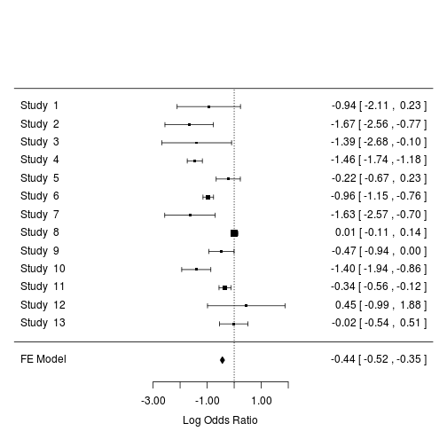

Customising the forest plot:

order: Sort by "obs", "fit", "prec", etc.
slab: Change study labels
ilab: Add study information
transf: Apply function to effects
psize: Symbol sizes

Order the studies by precision and transform log odds ratio to odds ratio:

forest(m2, order = "prec", transf = exp, refline = 1)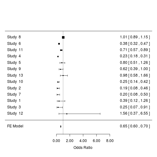

Add the sample size and year of the studies:

# sample size column to data
dat.bcg$n <- with(dat.bcg, tpos + tneg + cpos + cneg)

# plot
forest(m2, order = "prec", 
    ilab = dat.bcg[, c("n", "year")], 
    ilab.xpos = exp(m2$b) - c(4, 2), 
    transf = exp, refline = 1)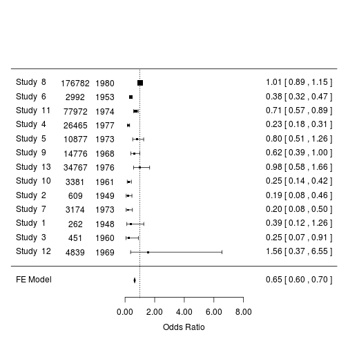

4. Meta-Regression With rma

Meta-regression is used to specify study covariates through the mods argument of rma.

The mods argument takes a matrix of p covariates.

m4 <- rma(ai = tpos, bi = tneg, ci = cpos, di = cneg, 
          data = dat.bcg, 
          mods = dat.bcg[, "ablat"], 
          measure = "OR", 
          method = "DL")

summary(m4)

## 
## Mixed-Effects Model (k = 13; tau^2 estimator: DL)
## 
##   logLik  deviance       AIC       BIC      AICc  
##  -7.4987   26.1043   20.9974   22.6922   23.6640  
## 
## tau^2 (estimated amount of residual heterogeneity):     0.0480 (SE = 0.0451)
## tau (square root of estimated tau^2 value):             0.2191
## I^2 (residual heterogeneity / unaccounted variability): 56.17%
## H^2 (unaccounted variability / sampling variability):   2.28
## R^2 (amount of heterogeneity accounted for):            86.90%
## 
## Test for Residual Heterogeneity: 
## QE(df = 11) = 25.0954, p-val = 0.0088
## 
## Test of Moderators (coefficient(s) 2): 
## QM(df = 1) = 26.1628, p-val < .0001
## 
## Model Results:
## 
##          estimate      se     zval    pval    ci.lb    ci.ub     
## intrcpt    0.3030  0.2109   1.4370  0.1507  -0.1103   0.7163     
## mods      -0.0316  0.0062  -5.1150  <.0001  -0.0437  -0.0195  ***
## 
## ---
## Signif. codes:  0 '***' 0.001 '**' 0.01 '*' 0.05 '.' 0.1 ' ' 1

5. Publication bias

It is possible that studies showing a significant intervention effect are more often published than studies with null results (the 'file drawer' problem).

When a meta-analysis is based only on studies reported in the literature, null studies relegated to the file-drawer could bias the summary intervention effect in the direction of efficacy

A funnel plot is a scatter plot of the intervention effect estimates against a measure of study precision.

Asymmetry (gaps) in the funnel may be indicative of publication bias.

Some authors argue that judging asymmetry is too subjective to be useful.

Spurious asymmetry can result from heterogeneity or when ESs are correlated with precision

funnel(m3)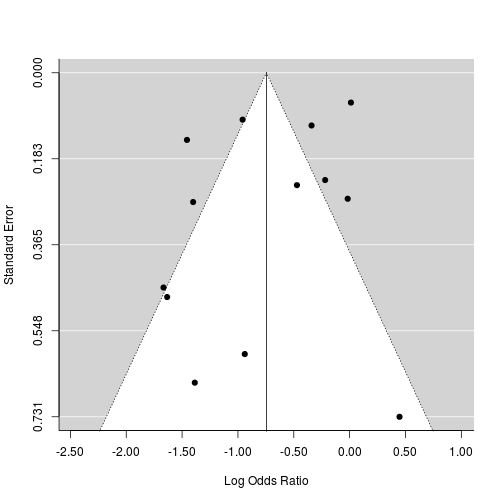

Acknowledgements

http://rpubs.com/skoval/meta

Links

https://ecologyforacrowdedplanet.wordpress.com/2013/05/10/using-metafor-and-ggplot-togetherpart-1/

http://ecologyforacrowdedplanet.wordpress.com/2013/05/30/using-metafor-and-ggplot-togetherpart-2/