Types of Data in R
R allows you to create new data structures
=======
Goals
-
Use different data modes.
-
Understand how the different data strutures are organised.
-
Create and subset these structures.
=======
Data objects in R can take one of certain forms.
These can be put together to create more complex objects.
Data objects can either be restricted to one kind of data, or contain more than one kind.
We will explore the common object types over the next few weeks.
=======
R has 5 different classes of data
Integer
x <- 1:10
Numeric
x <- c(1.5, 2.5, 3.34, 10.6576)
Character or string
simon_says <- c("hullo", "my", "name", "is", "Simon")
Logical
simon_says_again <- c("TRUE", "TRUE", "FALSE", "TRUE", "FALSE", "FALSE")
Complex (numbers with real and imaginary parts)
1 + 4i
=======
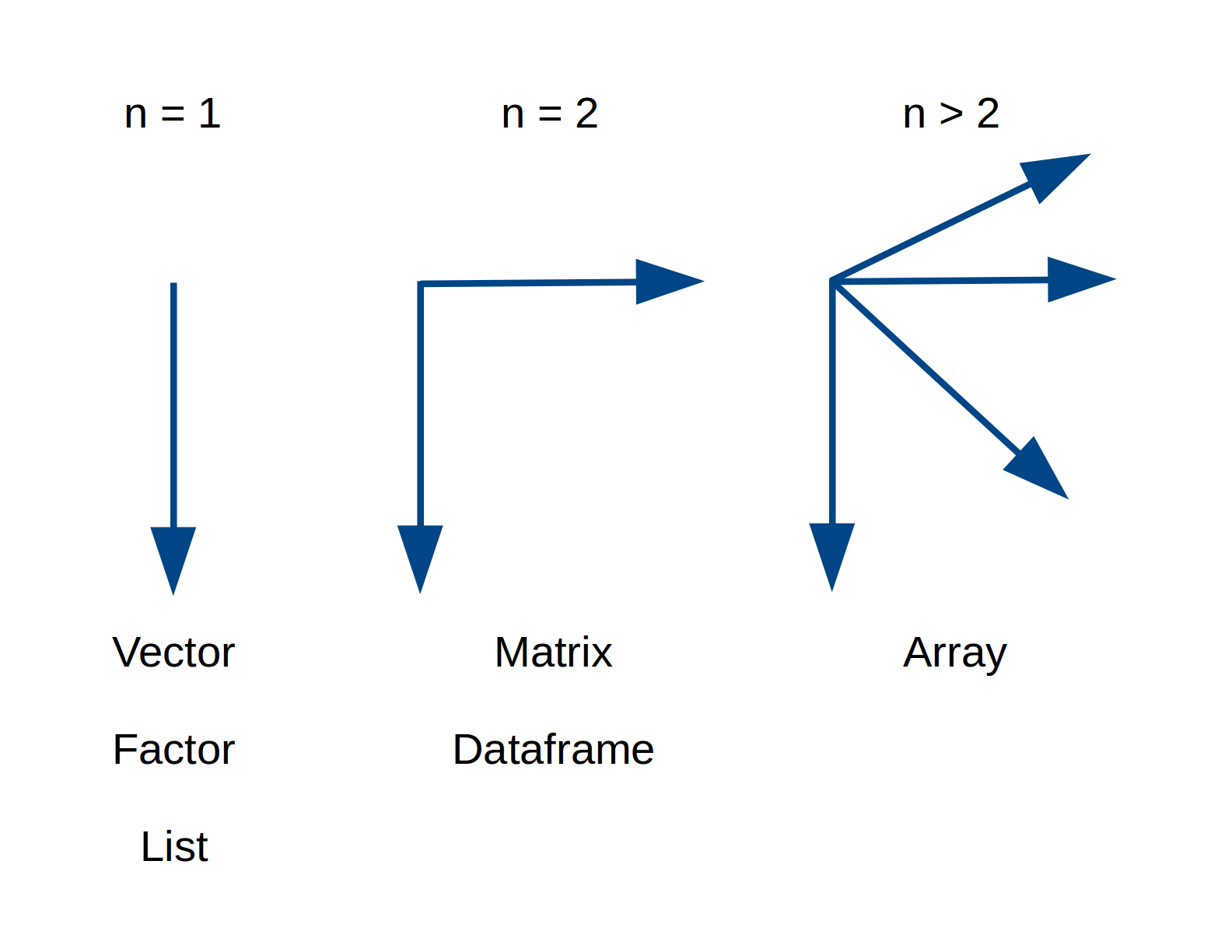
R has many different data structures
We can put data classes together in many different ways:
- vector
- matrix
- array
- factor
- dataframe
- list
======
Data objects have different dimensions
=======
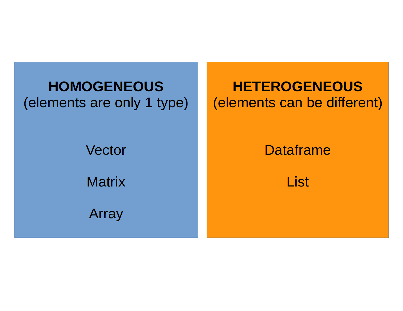
Data objects can be homogenous or heterogenous
=======
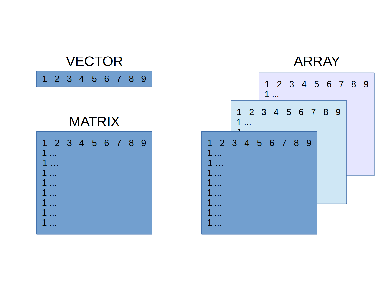
The simplest object is a vector
A vector can be thought of as equivalent to a single row or single column in a spreadsheet.
A vector is any number of elements stuck together.
x <- c(1, 2, 3, 4, 5, 6, 7, 8, 9, 10)
A single element is a vector of length 1.
x <- 1
A vector can contain only one class of data (= atomic vector).
All elements in a vector are coerced to be the same kind of data.
x <- c(1, 2, 3, 4, "a")
=======
A matrix is a 2D rectangular vector
Matrices are vectors with two dimensions.
Can be created by:
-
sticking vectors together,
-
chopping up a longer vector.
matrix(1:20, ncol = 5)
     [,1] [,2] [,3] [,4] [,5]
[1,]    1    5    9   13   17
[2,]    2    6   10   14   18
[3,]    3    7   11   15   19
[4,]    4    8   12   16   20
========
An array is a multi-dimensional collection of matrices
A 3D array in R:
> array(1:60, dim = c(4,5,3))
, , 1

     [,1] [,2] [,3] [,4] [,5]
[1,]    1    5    9   13   17
[2,]    2    6   10   14   18
[3,]    3    7   11   15   19
[4,]    4    8   12   16   20

, , 2

     [,1] [,2] [,3] [,4] [,5]
[1,]   21   25   29   33   37
[2,]   22   26   30   34   38
[3,]   23   27   31   35   39
[4,]   24   28   32   36   40

, , 3

     [,1] [,2] [,3] [,4] [,5]
[1,]   41   45   49   53   57
[2,]   42   46   50   54   58
[3,]   43   47   51   55   59
[4,]   44   48   52   56   60
=======
Vectors / Matrices / Arrays
=======
A factor is a vector that represents categorical data
Each element comes from a pre-defined set of categories.
Can be:
- ordinal (ordered or ranked): small, medium, large.
- nominal (unordered): blue, yellow, green
Factors can be written or coded using any mode (integer, text, logical).
=======
Factors can be unordered
# unordered 3-level factor with integers
x0 <- factor(c(1, 2, 3, 2))
x0
#[1] 1 2 3 2
#Levels: 1 2 3

table(x0)
#x0
#1 2 3
#1 2 1
=======
Factors can be unordered
# unordered 3-level factor with text (default order is alphanumeric)
x1 <- factor(c("large", "small", "medium", "small"))
x1
[1] large  small  medium small
Levels: large medium small

table(x1)
#x1
# large medium  small
#     1      1      2
========
Factors can be ordered
# ordered 3-level factor with text
x2 <- factor(c("large", "small", "medium", "small"),
             ordered = TRUE,
             levels = c("small", "medium", "large"))

x2
#[1] large  small  medium small
#Levels: small < medium < large

table(x2)
# small medium  large
#     2      1      1
=======
Dataframes can contain different kinds of data
Dataframes are equivalent to a single worksheet in a spreadsheet.
They can contain columns of different kinds of data.
You will likely read your data into R as a dataframe.
Year  Colour  Size_mm
2017  red     23.5
2016  red     12.67
2017  blue    15.2
2016  blue    1.0
...
=======
A List is a recursive vector
Lists can contain any other kind of data (including lists!) in a nested hierarchy.
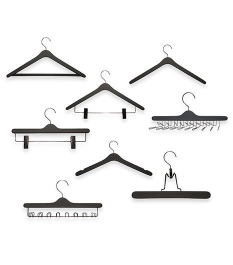
Lists are like a wardrobe (= closet) where you can store many different kinds of hangers and clothes:
- There is one main rail (hence it is 1D),
- You can hang any other object or class else on this rail,
- Including hanger with other rails (lists).
=======
R has many other data structures
-
Phylogenetic trees.
-
Vector GIS (shape files, …).
-
Spatial point pattern.
========
Code Glossary
In this appendix, we provide more details of the various data structure functions for future reference.
=======
1. Vectors
i). Creation
Make an empty vector.
x <- vector()
Specify the vector’s length.
x <- vector(length = 3)
The default mode is logical.
x
#[1] FALSE FALSE FALSE
ii). Tests
Is it a vector?
is.vector(x)
#[1] TRUE
What kind of vector?
is.numeric()
#[1] FALSE

is.character(x)
[1] FALSE

is.logical(x)
[1] TRUE
What is the vector’s length?
length(x)
#[1] 3
Structure of the vector?
str(x)
#logi [1:3] FALSE FALSE FALSE
Updated: 2017-09-14