Count data (Poisson)
Functions: glm()
A lot of data is in the form of counts (whole numbers or integers). For example, the number of species in plots, the number of sunny days per year, the number of restuarants in towns, ... With count data, the number 0 often appears as a value of the response variable.
Straightforward linear regression methods (assuming constant variance, normal errors) are not appropriate for count data for four main reasons:
The linear model might lead to the prediction of negative counts.
The variance of the response variable is likely to increase with the mean.
The errors will not be normally distributed.
Zeros are difficult to handle in transformations.
Poisson regression is used to model count variables.
The Poisson distribution was made famous by the Russian statistician Ladislaus Bortkiewicz (1868-1931), who counted the number of soldiers killed by being kicked by a horse each year in each of 14 cavalry corps in the Prussian army over a 20-year period. The data can be found here, if you are interested.
To fit a Poisson regression, we run a generalized linear model with family = poisson, which sets errors = Poisson and link = log. The log link ensures that all the fitted values are positive. The Poisson errors take account of the fact that the data are integer and have variances that are equal to their means.
We will illustrate a Poisson regression with data on the number of awards earned by students at one high school. Predictors of the number of awards earned include the type of program in which the student was enrolled (e.g., vocational, general or academic) and the score on their final exam in math.
dat <- read.table('../data/poisson-awards.txt', header = TRUE)
head(dat)
## student num_awards program math_score
## 1 1 0 vocational 40
## 2 2 0 vocational 33
## 3 3 0 academic 48
## 4 4 1 academic 41
## 5 5 1 academic 43
## 6 6 0 academic 46The response variable is the number of awards earned by each high-school student during the year ($num_awards). The predictor variables are each students' score on their math final exam ($math_score, continuous) and the type of program in which the students were enrolled ($program, categorical with three levels: general, academic, vocational).
summary(dat)## student num_awards program math_score
## Min. : 1.00 Min. :0.00 academic :105 Min. :33.00
## 1st Qu.: 50.75 1st Qu.:0.00 general : 45 1st Qu.:45.00
## Median :100.50 Median :0.00 vocational: 50 Median :52.00
## Mean :100.50 Mean :0.63 Mean :52.65
## 3rd Qu.:150.25 3rd Qu.:1.00 3rd Qu.:59.00
## Max. :200.00 Max. :6.00 Max. :75.00Checking the data
The Poisson distribution assumes that the mean and variance of the response variable, conditioned on the predictors, are equal. We can check this.
First, the unconditional mean and variance (i.e., the mean and variance of the whole vector).
mean(dat$num_awards)## [1] 0.63var(dat$num_awards)## [1] 1.108643Second, check the conditional mean and variance (i.e., the mean and variance of the respose variable conditional on the levels of categorical predictors).
They look pretty similar.
Me <- tapply(dat$num_awards, dat$program, mean)
Var <- tapply(dat$num_awards, dat$program, var)
rbind(Me, Var)
## academic general vocational
## Me 1.000000 0.2000000 0.2400000
## Var 1.634615 0.1636364 0.2677551We can also make a histogram of these data
barplot(t(table(dat$num_awards, dat$program)), beside = TRUE,
        xlab = 'Number of Awards', ylab = 'Count')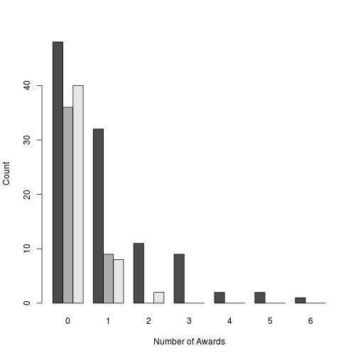
plot of chunk histogram-of-awards
Fitting the model
summary(m1 <- glm(num_awards ~ program + math_score,
                  family = 'poisson', data = dat))
##
## Call:
## glm(formula = num_awards ~ program + math_score, family = "poisson",
## data = dat)
##
## Deviance Residuals:
## Min 1Q Median 3Q Max
## -2.2043 -0.8436 -0.5106 0.2558 2.6796
##
## Coefficients:
## Estimate Std. Error z value Pr(>|z|)
## (Intercept) -4.16327 0.66288 -6.281 3.37e-10 ***
## programgeneral -1.08386 0.35825 -3.025 0.00248 **
## programvocational -0.71405 0.32001 -2.231 0.02566 *
## math_score 0.07015 0.01060 6.619 3.63e-11 ***
## ---
## Signif. codes: 0 '***' 0.001 '**' 0.01 '*' 0.05 '.' 0.1 ' ' 1
##
## (Dispersion parameter for poisson family taken to be 1)
##
## Null deviance: 287.67 on 199 degrees of freedom
## Residual deviance: 189.45 on 196 degrees of freedom
## AIC: 373.5
##
## Number of Fisher Scoring iterations: 6Call: The model
Deviance Residuals: Deviance residuals are approximately normally distributed if the model is specified correctly. Here, it shows a little bit of skeweness since median is not quite zero.
Coefficients: The Poisson regression coefficients, standard errors, z-scores, and p-values for each variable.
For continuous predictor variables, the coefficient estimate is the expected log count of the response variable for a one-unit increase in a continuous predictor. For example, the coefficient for $math_score is 0.07. This means that the expected increase in log award number for a one-unit increase in math is 0.07.
For categorical predictor variables, the coefficient estimate is the expected difference in log count between the baseline level (in this case, academic) and each other level. For example, the expected difference in log count for general compared to academic is -1.08. The expected difference in log count for vocational compared to academic is -0.7: students in general and vocation programs got fewer awards than students in academic programs.
Deviance: The residual deviance can be used to test for the goodness of fit of the overall model. The residual deviance is the difference between the deviance of the current model and the maximum deviance of the ideal model where the predicted values are identical to the observed. The smaller the residual deviance, the better the model fit.
First, we can eyeball this by checking if the residual deviance is similar to the residual degrees of freedom (it should be, because the variance and the mean should be the same). If the residual deviance is larger than residual degrees of freedom, this suggests that there is extra, unexplained variation in the response (overdispersion). Overdispersion can be compensated for by refitting the model using quasi-Poisson rather than Poisson errors.
Second, we can explicitly run a goodness-of-fit test.
pchisq(m1$deviance, m1$df.residual, lower.tail = FALSE)## [1] 0.6182274If the residual difference is small enough, the goodness of fit test will not be significant, indicating that the model fits the data.
We can test the overall effect of $program by comparing the deviance of the full model with the deviance of the model excluding $program.
## make new model without program
m2 <- glm(num_awards ~ math_score,
          family = 'poisson', data = dat)
## test model differences with chi square test
anova(m2, m1, test = "Chisq")
## Analysis of Deviance Table
##
## Model 1: num_awards ~ math_score
## Model 2: num_awards ~ program + math_score
## Resid. Df Resid. Dev Df Deviance Pr(>Chi)
## 1 198 204.02
## 2 196 189.45 2 14.572 0.0006852 ***
## ---
## Signif. codes: 0 '***' 0.001 '**' 0.01 '*' 0.05 '.' 0.1 ' ' 1The two degree-of-freedom chi-square test indicates that $program is a statistically significant predictor of num_awards.
Plotting the model
We first need to calculate and store predicted values for each row in the original dataset (we have enough data here that, at least for our purposes, we do not need to generate a new vector of math_scores).
dat$phat <- predict(m1, type = "response")To plot them, we need to order the data by $program and $math_score
dat2 <- dat[order(dat$program, dat$math_score), ]Now, we can plot the data points (adding some jitter to the counts), and add the predicted lines.
plot(jitter(dat$num_awards) ~ math_score, data = dat, col = program, pch = 20)
lines(phat ~ math_score, data = dat2[dat2$program == 'academic', ])
lines(phat ~ math_score, data = dat2[dat2$program == 'general', ], col = 2)
lines(phat ~ math_score, data = dat2[dat2$program == 'vocational', ], col = 3)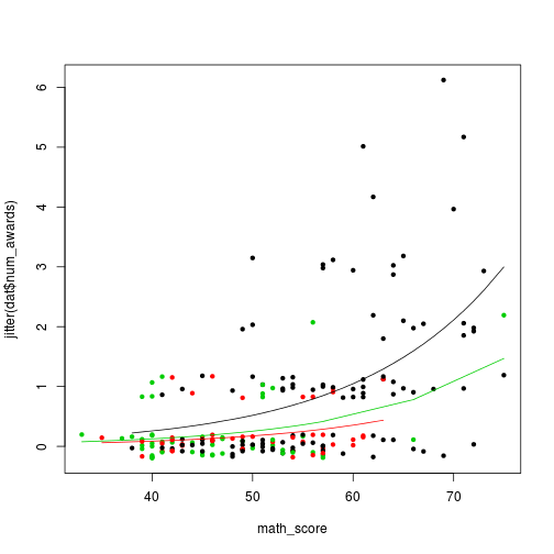
plot of chunk plotting-count-data
Note: In the call to predict(), we could leave out ```type = "response". This would generate predicted values on the log scale, and we would need to antilog (exponentiate) them to get counts.
dat$phat.log <- predict(m1)
dat$phat.exp <- exp(dat$phat.log)
head(dat)
## student num_awards program math_score phat phat.log
## 1 1 0 vocational 40 0.12603202 -2.0712193
## 2 2 0 vocational 33 0.07712822 -2.5622861
## 3 3 0 academic 48 0.45115236 -0.7959502
## 4 4 1 academic 41 0.27609315 -1.2870170
## 5 5 1 academic 43 0.31767953 -1.1467122
## 6 6 0 academic 46 0.39209349 -0.9362550
## phat.exp
## 1 0.12603202
## 2 0.07712822
## 3 0.45115236
## 4 0.27609315
## 5 0.31767953
## 6 0.39209349Exercises
Disease as a function of distance from a potential source
clusters <- read.table("../data/clusters.txt", header = TRUE)
head(clusters)
## Cancers Distance
## 1 0 11.46952
## 2 0 66.55395
## 3 0 47.46230
## 4 0 48.38129
## 5 0 73.76534
## 6 0 70.57555hist(clusters$Cancers)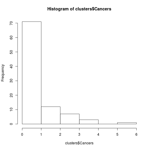
Fig. Histogram of some count data
Model $Cancers as a function of $Distance.
Plot the data and predicted line.
Prussian horse-kick data
Load the famous data. It shows the number of deaths from horse-kicks in each of 16 different companies in the Prussian army from 1875 to 1894.
dat <- read.table('http://www.math.uah.edu/stat/data/HorseKicks.txt', header = TRUE)
head(dat)
## Year GC C1 C2 C3 C4 C5 C6 C7 C8 C9 C10 C11 C14 C15
## 1 1875 0 0 0 0 0 0 0 1 1 0 0 0 1 0
## 2 1876 2 0 0 0 1 0 0 0 0 0 0 0 1 1
## 3 1877 2 0 0 0 0 0 1 1 0 0 1 0 2 0
## 4 1878 1 2 2 1 1 0 0 0 0 0 1 0 1 0
## 5 1879 0 0 0 1 1 2 2 0 1 0 0 2 1 0
## 6 1880 0 3 2 1 1 1 0 0 0 2 1 4 3 0Test whether there were differences in the number of deaths between companies.
Was any year particularly bad for deaths?
Updated: 2017-11-08