GLMs: Binomial data
Functions: glm()
Many statistical problems involve binary response variables. For example, we could classify individuals as alive/dead, healthy/unwell, employ/unemployed, left/right, right/wrong, ... etc. A regression of binary data is possible if at least one of the predictors is continuous (otherwise you would use some kind of categorical test, such as a Chi-squared test).
The response variable contains only 0s and 1s (e.g., dead = 0, alive = 1) in a single vector. R treats such binary data is if each row came from a binomial trial with sample size 1. If the probability that an individual is dead is p, then the probability of obtaining y (where y is either dead or alive, 0 or 1) is given by an abbreviated form of the binomial distribution with n = 1, known as the Bernoulli distribution.
Binomial data can either be modelled at the individual (binary response) or group (proportion) level. If you have unique values of one or more explanatory variables for each and every individual case, then a model with a binary response variable will work. If not, you should aggregate the data until you do have such explanatory variables (e.g., at the level of the household, town, state, population, ...).
Individual-level: binary response (0/1): logistic regression
At the individual level we can model each individual in terms of dead or alive (male/female, tall/short, green/red, ...), using logistic regression (or logit model). In the logit model, the log odds (logarithm of the odds) of the outcome is modeled as a linear combination of the predictor variables. If p is a probability, then p/(1 − p) is the corresponding odds; the logit of the probability is the logarithm of the odds.
To model a binary response variable, we first need (or need to create) a single vector of 0 and 1s. We model this with glm() and family = 'binomial'. We can compare models using a test for a change in deviance with chi-squared. Overdispersion is not an issue with a binary response variable.
Let's look at the incidence (presence/absence) of a breeding bird on various islands.
isol <- read.table("../data/isolation.txt", header = TRUE)
head(isol)
## incidence area isolation
## 1 1 7.928 3.317
## 2 0 1.925 7.554
## 3 1 2.045 5.883
## 4 0 4.781 5.932
## 5 0 1.536 5.308
## 6 1 7.369 4.934The data show the $incidence of the bird (present = 1, absent = 0) on islands of different sizes ($area in km2) and distance ($isolation in km) from the mainland.
We begin by fitting a complex model involving an interaction between isolation and area:
model1 <- glm(incidence ~ area * isolation, family = binomial, data = isol)Then we fit a simpler model with only main effects for isolation and area:
model2 <- glm(incidence ~ area + isolation, family = binomial, data = isol)We now can compare the two models using ANOVA. In the case of binary data, we need to do a Chi-squared test.
anova(model1, model2, test = "Chi")## Analysis of Deviance Table
##
## Model 1: incidence ~ area * isolation
## Model 2: incidence ~ area + isolation
## Resid. Df Resid. Dev Df Deviance Pr(>Chi)
## 1 46 28.252
## 2 47 28.402 -1 -0.15043 0.6981summary(model2)##
## Call:
## glm(formula = incidence ~ area + isolation, family = binomial,
## data = isol)
##
## Deviance Residuals:
## Min 1Q Median 3Q Max
## -1.8189 -0.3089 0.0490 0.3635 2.1192
##
## Coefficients:
## Estimate Std. Error z value Pr(>|z|)
## (Intercept) 6.6417 2.9218 2.273 0.02302 *
## area 0.5807 0.2478 2.344 0.01909 *
## isolation -1.3719 0.4769 -2.877 0.00401 **
## ---
## Signif. codes: 0 '***' 0.001 '**' 0.01 '*' 0.05 '.' 0.1 ' ' 1
##
## (Dispersion parameter for binomial family taken to be 1)
##
## Null deviance: 68.029 on 49 degrees of freedom
## Residual deviance: 28.402 on 47 degrees of freedom
## AIC: 34.402
##
## Number of Fisher Scoring iterations: 6The simpler model is not significantly worse, so we can go with that one.
Fitting and interpreting the model
summary(model2)##
## Call:
## glm(formula = incidence ~ area + isolation, family = binomial,
## data = isol)
##
## Deviance Residuals:
## Min 1Q Median 3Q Max
## -1.8189 -0.3089 0.0490 0.3635 2.1192
##
## Coefficients:
## Estimate Std. Error z value Pr(>|z|)
## (Intercept) 6.6417 2.9218 2.273 0.02302 *
## area 0.5807 0.2478 2.344 0.01909 *
## isolation -1.3719 0.4769 -2.877 0.00401 **
## ---
## Signif. codes: 0 '***' 0.001 '**' 0.01 '*' 0.05 '.' 0.1 ' ' 1
##
## (Dispersion parameter for binomial family taken to be 1)
##
## Null deviance: 68.029 on 49 degrees of freedom
## Residual deviance: 28.402 on 47 degrees of freedom
## AIC: 34.402
##
## Number of Fisher Scoring iterations: 6As normal, we have the formula, the deviance residuals (a measure of model fit), then the coefficient estimates, their standard errors, the z-statistic (sometimes called a Wald z-statistic), and p-values.
Logit/log odds
The logistic regression coefficients give the change in the log odds (the logarithm of the odds, or logit).
For continuous predictors, the coefficients give the change in the log odds of the outcome for a one unit increase in the predictor variable. For example, for every 1km2 increase in area, the log odds of the bird being present (versus absent) increases by 0.58 and the log odds of the bird being present decreases by 1.37 (i.e., -1.37) for every km of distance from the mainland.
For categorical predictors, the coefficient estimate describes the change in the log odds for each level compared to the base level.
Confidence intervals around the logits can be calculated with confint().
confint(model2)## Waiting for profiling to be done...## 2.5 % 97.5 %
## (Intercept) 1.8390115 13.735103
## area 0.1636582 1.176611
## isolation -2.5953657 -0.639140Logits (log odds) are just one way of describing the model. We can easily convert the logits either to odds ratios or predicted probabilities.
Odds ratios
Odds ratios are a relative measure of effect, which allows the comparison of two groups. It is a popular way of presenting results in medicine, especially of controlled trials. Here, the odds of one group (usually the control) is divided by the odds of another (the treatment) to give a ratio. In this case, if the odds of both groups are the same, the ratio will be 1, suggesting there is no difference. If the OR is > 1 the control is better than the other level. If the OR is < 1 the treatment is better than the control.
However, in R, we are presented with differences or the change in log odds between groups (for categorical variables) or the change in log odds between x and x + 1 (for continuous variables). The directionality is the opposite to the example above because R effectively compares the 'treatment' to the 'control'.
Thus, for categorical predictors, an odds ratio of > 1 suggests a positive difference between levels and the base level (the exponential of a positive number is greater than 1), i.e., the base level has a lower odds and the level has a higher odds. An odds ratio of < 1 suggests a negative difference (the exponential of a negative number lies between 0 and 1).
For continuous predictors, the odds ratio is the odds of x + 1 over x (i.e., the odds ratio for a unit increase in the continuous x predictor variable), and the interpretation is the same as for categorical.
exp(coef(model2))## (Intercept) area isolation
## 766.3669575 1.7873322 0.2536142See http://www.ats.ucla.edu/stat/mult_pkg/faq/general/odds_ratio.htm for more details.
Predicted probabilities
We can generate predicted probabilities for continuous and categorical variables.
We can generate predicted probabilities for each row in the original dataset, just be calling the predict() function.
Setting type = 'link' returns the logits; setting type = 'response' returns the predicted probabilities.
isol$logit <- predict(model2, type = 'link')
isol$p <- predict(model2, type = 'response')
However, to better plot these relationships, we should input a specific range of x's that we predict y's for.
Plotting binary response data
To plot the fitted line of a generalized linear model, we generally have to use the predict() function, because the model, although linear, is not a straight line that can be plotted with either an intercept or slope, as we used for lm() and abline().
The function predict() is a general wrapper for more specific functions, in this case predict.glm(). We have to specific the object (i.e., the fitted model), the newdata (i.e., the values of x for which we want predictions, named identically to the predictors in the object), and the type of prediction required (either on the scale of the linear predictors ('link') or on the scale of the response variable ('response').
There are, as usual, at least two ways we could do this.
First, we will make two separate individual logistic regressions and make predictions from those.
# run two models, one for area and one for isolation
modela <- glm(incidence ~ area,      family = binomial, data = isol)
modeli <- glm(incidence ~ isolation, family = binomial, data = isol)
We then need to make a sequence of x (e.g., $area) values from which to predict the y (predicted probability of $incidence).
# create a sequence of x values
xv <- seq(from = 0, to = 9, by = 0.01)

# y values
yv <- predict(object = modela, newdata = list(area = xv), type = "response")
Now, we have two vectors, xv and yv, that we can use to plot the fitted line.
# set up a two-panel plotting area
par(mfrow = c(1, 2))

 ## 1. area
 # plot the raw data
   plot(isol$area, isol$incidence)

 # use the lines function to add the fitted lines
   lines(xv, yv)

  ## 2. Now, repeat for isolation
  xv2 <- seq(0, 10, 0.1)
  yv2 <- predict(modeli, list(isolation = xv2),type = "response")
  plot(isol$isolation, isol$incidence)
  lines(xv2, yv2)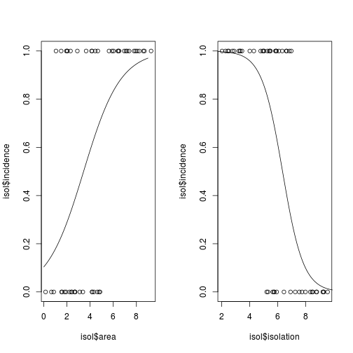
Fig. Plotting binary response variables
Alternatively, we could use the original model2 and generate values for the range of $area contingent on the mean value of $isolation, and vice versa.
# Generate a sequence of x's from which to make predictions. Because area and isolation are on similar scales, we can use the same sequence for both.
x.seq <- seq(from = 0, to = 9, by = 0.1)

# make a new dataframe, of x.seq for area and x.seq for isolation, along with the mean of the corresponding column
xv3 <- data.frame(area = c(x.seq, rep(mean(isol$area), times = length(x.seq))), isolation = c(rep(mean(isol$isolation), times = length(x.seq)), x.seq ))

# Use predict() on the new dataframe
# (in this case, we do not need to make it into a list)
xv3$y <- predict(model2, newdata = xv3, type = 'response')

head(xv3)
## area isolation y
## 1 0.0 5.8563 0.1989551
## 2 0.1 5.8563 0.2083722
## 3 0.2 5.8563 0.2181137
## 4 0.3 5.8563 0.2281793
## 5 0.4 5.8563 0.2385677
## 6 0.5 5.8563 0.2492763We could then plot y on area and y on isolation using lines(), as above.
Group-level: Proportion data
At the group level, we look at the proportion of successes and failures (or male/famale, tall/short, dem/rep, ...) in groups/populations/sites. In all these cases, we know both numbers ... those of successes and those of failures, in contrast to Poisson regression where we just have counts of successes.
In the past, the way this data was modelled was to use a single percentage as the response variable. However, this causes problems because:
The errors are not normally distributed.
The variance is not constant.
The response is bounded (by 1 above and by 0 below).
We lose information on the size of the sample, n, from which the proportion was estimated.
In the GLM framework, we can model proportion data directly. R carries out weighted regression, using the individual sample sizes as weights, and the logit link function to ensure linearity.
Overdispersion
Overdispersion occurs in regression of proportion data when the residual deviance is larger than the residual degrees of freedom. There are two possibilities: either the model is misspecified, or the probability of success, p, is not constant within a given treatment level.
To deal with overdispersion, we can set family = quasibinomial rather than family = binomial.
Fitting the model
As above, we use glm() with family = 'binomial'. In contrast to the binomial response, in the case of proportion data, our response data is a matrix of two columns, one column of successes and one of failures. This matrix must be single object (i.e., you could use cbind() to stick two columns together), which in most cases we will call y.
In this case, we have the number of males and females in a range of populations. Does sex ratio vary with population size?
numbers <- read.table("../data/sexratio.txt", header = TRUE)
head(numbers)
## density females males
## 1 1 1 0
## 2 4 3 1
## 3 10 7 3
## 4 22 18 4
## 5 55 22 33
## 6 121 41 80To model proportion data, R requires a unique form of the response variable - a matrix of two columns of successes and failures, in this case males and females.
numbers$p <- numbers$males/(numbers$males + numbers$females)
y <- cbind(numbers$males, numbers$females)
y
## [,1] [,2]
## [1,] 0 1
## [2,] 1 3
## [3,] 3 7
## [4,] 4 18
## [5,] 33 22
## [6,] 80 41
## [7,] 158 52
## [8,] 365 79We specifiy the model as follows.
m1 <- glm(y ~ numbers$density, family = binomial)
summary(m1)
##
## Call:
## glm(formula = y ~ numbers$density, family = binomial)
##
## Deviance Residuals:
## Min 1Q Median 3Q Max
## -3.4619 -1.2760 -0.9911 0.5742 1.8795
##
## Coefficients:
## Estimate Std. Error z value Pr(>|z|)
## (Intercept) 0.0807368 0.1550376 0.521 0.603
## numbers$density 0.0035101 0.0005116 6.862 6.81e-12 ***
## ---
## Signif. codes: 0 '***' 0.001 '**' 0.01 '*' 0.05 '.' 0.1 ' ' 1
##
## (Dispersion parameter for binomial family taken to be 1)
##
## Null deviance: 71.159 on 7 degrees of freedom
## Residual deviance: 22.091 on 6 degrees of freedom
## AIC: 54.618
##
## Number of Fisher Scoring iterations: 4The output is familar. For this continuous predictor, we get an intercept and slope, and the p-values indicate whether they are significantly different from 0.
For categorical variables, we get, as usual, the base level mean, then differences between means. Furthermore, the coefficient estimates are in logits (ln(p/(1 - p)). To calculate a proportion (p) from a logit (x), you need to calculate 1/(1 + 1/(exp(x))).
However, we have substantial overdispersion (residual deviance = 22.091 is much greater than residual d.f. = 6). One reason for overdispersion is if the model is misspecified. Let's try log(density).
m2 <- glm(y ~ log(density), family = binomial, data = numbers)
summary(m2)
##
## Call:
## glm(formula = y ~ log(density), family = binomial, data = numbers)
##
## Deviance Residuals:
## Min 1Q Median 3Q Max
## -1.9697 -0.3411 0.1499 0.4019 1.0372
##
## Coefficients:
## Estimate Std. Error z value Pr(>|z|)
## (Intercept) -2.65927 0.48758 -5.454 4.92e-08 ***
## log(density) 0.69410 0.09056 7.665 1.80e-14 ***
## ---
## Signif. codes: 0 '***' 0.001 '**' 0.01 '*' 0.05 '.' 0.1 ' ' 1
##
## (Dispersion parameter for binomial family taken to be 1)
##
## Null deviance: 71.1593 on 7 degrees of freedom
## Residual deviance: 5.6739 on 6 degrees of freedom
## AIC: 38.201
##
## Number of Fisher Scoring iterations: 4There is no evidence of overdispersion (residual deviance = 5.67 on 6 d.f.) in this new model.
We can conclude that the proportion of males increases significantly with increasing density, and that the logistic model is linearized by logarithmic transformation of the explanatory variable (population density).
Plotting proportion data
We plot the proportion of males.
# make sequence of x
xv <- seq(from = 0, to = 6, by = 0.01)

# predict values of y from xv and m2
yv <- predict(m2, list(density = exp(xv)), type = "response")

# plot the proportion of males as a function of density
plot(x = log(numbers$density), y = numbers$p, ylab = "Proportion male",
     pch = 16, col = "blue", lwd = 2)

# add the fitted line
lines(xv, yv, col = "red", lwd = 2)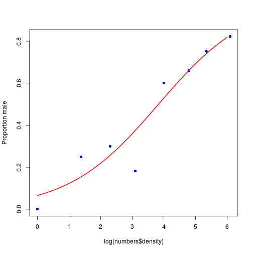
Fig. Plotting proportion data
Note: Some kinds of proportion data are better analysed differently.
Percentage cover is best analysed using conventional linear models (assuming normal errors and constant variance) following arcsine transformation.
Percentage change in some continuous measurement (e.g., weight, tree diameter) is best modelled either as an ANCOVA of the final measurement with the initial measurement as a covariate, or by specifying the response as a relative change: log(final/initial), both of which should be linear models with normal errors.
Exercises
Individual Voting in the 2004 Presidential Election
Andrew Gelman, Boris Shor, Joseph Bafumi and David Park (2008), "Rich State, Poor State, Red State, Blue State: What's the Matter with Connecticut?", Quarterly Journal of Political Science: Vol. 2: No. 4, pp 345-367. http://dx.doi.org/10.1561/100.00006026
For decades, the Democrats have been viewed as the party of the poor, with the Republicans representing the rich. Recent presidential elections, however, have shown a reverse pattern, with Democrats performing well in the richer blue states in the northeast and coasts, and Republicans dominating in the red states in the middle of the country and the south.
We will use the National Annenberg Election Survey data to examine the predictors of voting patterns.
The National Annenberg Election Survey (NAES) examines a wide range of political attitudes about candidates, issues and the traits Americans want in a president. It also has a particular emphasis on the effects of media exposure through campaign commercials and news from radio, television and newspapers. Additionally, it measures the effects of other kinds of political communication, from conversations at home and on the job to various efforts by campaigns to influence potential voters.
We will look at the 2004 US Presidential Election
The data are available here, or as supplemental data from Gelman et al. (2008).
The data are a STATA data file. You will need to install the 'foreign' R package to be able to use the read.dta() function to read in the data.
library(foreign)
dat1 <- read.dta('../data/annen2004_processed.dta', convert.factors = FALSE)

# setting 'convert.factors = TRUE' keeps the original text in the columns
dat2 <- read.dta('../data/annen2004_processed.dta', convert.factors = TRUE)

head(dat2)
The column $votechoice is the binomial response variable: 0 = democrat (Kerry), 1 = republican (Bush).
Examine the data.
What factors predicted a person's vote?
Did these factors vary by state?
How accurate are the polls? The 2008 US Presidential Election
The US presidential election is held every four years on Tuesday after the first Monday in November. The 2016 presidential election date is scheduled for Nov 8, 2016. The 2008 and 2012 elections were held, respectively, on Nov 4, 2008 and Nov 6, 2012. The President of US is not elected directly by popular vote. Instead, the President is elected by electors who are selected by popular vote on a state- by-state basis. These selected electors cast direct votes for the President. Almost all the states except Maine and Nebraska, electors are selected on a “winner- take-all” basis. That is, all electoral votes go to the presidential candidate who wins the most votes in popular vote. For simplicity, we will assume all the states use the “winner-take-all” principle in this lab. The number of electors in each state is the same as the number of congressmen of that state. Currently, there are a total of 538 electors including 435 House representatives, 100 senators and 3 electors from the District of Columbia. A presidential candidate who receives an absolute majority of electoral votes (no less than 270) is elected as President. For simplicity, our data analysis only considers the two major political parties: Democratic (Dem) and Republican (Rep). The interest is to predict which party (Dem or Rep) will win the most votes in each state. Because the chance that a third-party (except Dem and Rep) receives an electoral vote is very small, our simplification is reasonable.
Prediction of the outcomes of presidential election campaigns is of great interests to many people. In the past, the prediction was typically made by political analysts and pundits based on their personal experience, intuition and preferences. However, in recent decades, statistical methods have been widely used in predicting election results. Surprisingly, in 2012, statistician Nate Silver correctly predicted the outcome in every state while he successfully called the outcomes in 49 states out of the 50 states in 2008.
The data come from the 2008 polling and election.
The original data can be found here: 2008 polling 2008 election
These datasets give the percentage of Dem and Rep votes for each state.
However, we will use a combined and modifed version of these data, to test whether the polling was accurate.
Our data can be downloaded from here. It contains five columns: whether the poll was correct ($resp), the state ($statesFAC), the difference between Dem and Rep result ($margins), the time before the election ($lagtime), and the pollster (polsterFAC).
How accurate were the polls?
How did the margins and lagtime affect their prediction?
Quiz
Using the National Election Survey data from the first exercise (2004 Annenberg Election Survey)...
Plot the relationship between the probability of voting Republican and a voter's age.
Plot the relationship between the probability of voting Republican and a voter's age, with a line for each sex.
There are a couple of issues with this dataset.
The
$agecolumn has some missing data (represented by999). You will need to deal with these.The
$votechoicecolumn has some missing data (represented byNA), but this will not affect the model or plots.
Make sure that you work through the Poisson page example before working on thes questions. That example will help with using predict().
Updated: 2017-11-09