Data Exploration, or rubbish in, rubbish out
Functions:
A Protocol for Data Exploration to Avoid Common Statistical Problems
Zuur et al. 2010 Methods in Ecology & Evolution
doi: doi: 10.1111/j.2041-210X.2009.00001.x
Overview
The analyses in many reports and published papers do not meet the underlying assumptions of the statistical techniques employed. Some techniques are more robust than others, and some of these violations have little or no impact on the results. But other violations increase Type I or Type II errors, leading to the wrong conclusions.
Here, we look at (mostly graphical) checks for the common problems.
#dat <- read.table(file = "http://www.simonqueenborough.info/R/data/sparrows.txt", header = TRUE)
dat <- read.table('~/Dropbox/MyLab/website/R/data/sparrows.txt', header = TRUE, sep = '\t')
1. Outliers in y and x
Some analyses are more or less sensitive to the presence of observations with a relatively larger or smaller value than most of the data. They could come from a variety of sources, but in general should not be deleted from the data.
To identify outliers, we can use boxplots ...
boxplot(dat$Wingcrd)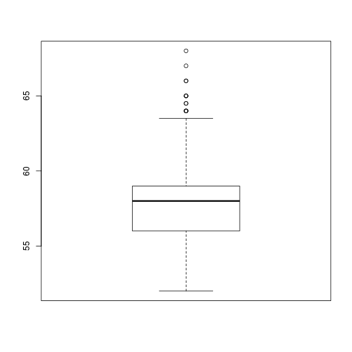
plot of chunk unnamed-chunk-2
... or Cleveland dotplots.
par(mfrow = c(1,2), lwd = 2)
dotchart(dat$Wingcrd, lcolor = 0)
dotchart(sort(dat$Wingcrd), lcolor = 0)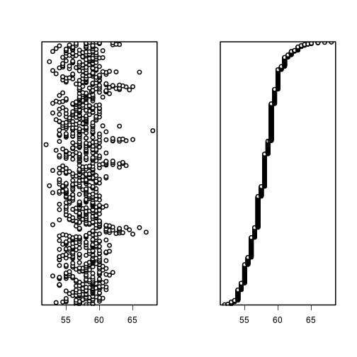
plot of chunk unnamed-chunk-3
Solution: outliers due to measurement, data transcription, or other human error can either be corrected, or dropped, programmatically. Otherwise, understanding what may have caused them is important.
2. Homogeneity of y
Homogeneity of variance is an important assumption in ANOVA, other regression-related models and in multivariate techniques such as discriminant analysis. In ANOVA, this means that the variation in observations between and across groups should be similar. In regression, the residuals should be tested.
# Do males and females have similar variance in Head size?
boxplot(dat$Head ~ dat$Sex)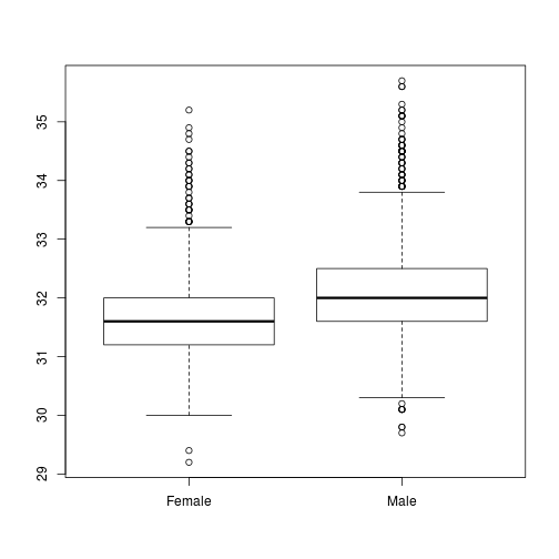
Fig. Head size versus Sex
Solution: transform the response variable to stabilize the variance, or apply a statistical technique that does not require homogeneity (e.g., gls).
3. Normality of y
A number of statistical methods have an assumption of normality (e.g., linear regression, t-tests); others do not (PCA).
Some techniques are robust to violating this assumption (e.g., linear regression).
For t-tests and ANOVA that assume normality, histograms of the data should be made.
For linear regression, the assumption is that each observation is drawn from a normal distribution around each covariate value. This assumption is usually impossible to test directly, but normality of the residuals (via a histogram after constructing the model) would support this assumption.
Solution: Transformation may help; otherwise a (no-parametric) test that has no assumption of normality.
4. Lots of 0's in y
A large number of 0's in the observations (e.g., in counts of individuals or species) can lead to biased parameter estimates and standard errors.
Solution: Zero-inflated distributions (especially for generalised linear models) that should be used instead.
5. Collinearity in the x covariates
Collinearity is the existence of correlation between covariates.
Collinearity can occur in a variety of situations, including:
- if measurements are taken from the same individual (e.g., height and weight are often correlated),
- analyses where different predictors would sum to 100 (e.g., % ground cover by shrubs, % ground cover by herbs),
- many measurements are taken (e.g., soil biogeochemistry),
- if spatial or temporal variation correlated with other measurements (e.g., rainfall and temperature with latitude or elevation).
Collinearity can be a problem in multiple linear regression, ANOVA, GLMs, GAMs, and mixed effects models, as well as multivariate models such as RDA and CCA.
Collinearity causes problems, because correlated variables 'steal' statistical information from one another, often leading to a confused statistical analysis where nothing is significant and where dropping one covariate has a large effect, even changing the sign of other parameters.
Collinearity can be detected by plotting all variables against each other, using plot():
# here, we plot all the sparrow data
plot(dat)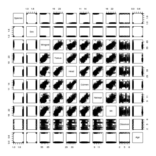 Many of the continuous variables are correlated; this collinearity can be tested with correlation coefficients, scatterplots or PCA biplots. Note that estimates of collinearity (e.g., Pearson correlation coefficient) can be affected by outliers.
Solution: Drop correlated predictors (use common sense or theory).
6. What are the relationships in y and x
The response variable should be plotted against each predictor (boxplots, dotplots, scatterplots, ...).
Just because no clear patterns are obvious between the response and any covariate does not indicate that there are no relationships. A model with multiple explanatory variables may still provide a good fit.
7. Interactions
Are they any interactions between the x variables? For example, do any of the continuous predictors vary with categorical predictors?
8. Independence of y
We touched on this issue already in which test.
A critical assumption of most statistical tests is that observations are independent of one another. If observations are auto-correlated it means that information on one observation provides information about other observations after the effects of other variables have been accounted for.
Independence of observations is especially important for regression, and violation can lead to vastly inflated p-values, increasing type I error (false positive).
Observations can be autocorrelated in space, time, ancestry/relatedness, or sequence. If there is some autocorrelation in the residuals of the model, this needs to be accounted for. There are various ways to do this.
Updated: 2016-10-15