Community ordination methods
We often have large data sets of different observations or measurements from the same sampling units or sites.
For example, we may have a network of quadrats, plots, or sites with incidence or abundance data on taxa present at each site, along with environmental variables (soil nutrients, elevation, aspect, ...). Or, we may have measurements of many different variables from the same individuals or sampling units (e.g., individual sparrows).
A good resource: http://ordination.okstate.edu/overview.htm
There are several reasons to use ordination:
Reducing the number of potentially correlated dependent variables (e.g., soil nutrients, multiple variables on the same individuals).
Modelling occurance of a large number of species that would be hard to model individually.
Both are exemplified by John et al. 2007
Ordination in R
There are a large number of different ordination methods that are each slightly and subtley different, and best-used in specific situations.
These methods include principle components analysis, principle coordinates analysis, non-metric multi-dimensional scaling, detrended correspondance analysis, canonical correspondance analysis, ...
Read the help files, vegan tutorials, etc. if you are planning on doing an ordination to ensure that you use the most appropriate method/s.
Basic ordination methods are available in base R, and there are a number of specialist packages that extend these capabilities.
Two main packages in R:
Simple ordination
Using the sparrow data, we can use PCA to ask whether there are general differences between species or sex.
dat <- read.table(file = "http://www.simonqueenborough.info/R/data/sparrows.txt", header = TRUE)
head(dat)
## Species Sex Wingcrd Tarsus Head Culmen Nalospi Wt Observer Age
## 1 SSTS Male 58.0 21.7 32.7 13.9 10.2 20.3 2 0
## 2 SSTS Female 56.5 21.1 31.4 12.2 10.1 17.4 2 0
## 3 SSTS Male 59.0 21.0 33.3 13.8 10.0 21.0 2 0
## 4 SSTS Male 59.0 21.3 32.5 13.2 9.9 21.0 2 0
## 5 SSTS Male 57.0 21.0 32.5 13.8 9.9 19.8 2 0
## 6 SSTS Female 57.0 20.7 32.5 13.3 9.9 17.5 2 0Base R (in the stats package) has two functions to calculate a Principle Components Analysis (PCA), prcomp() and princomp().
Using prcomp() returns the pca axes for each variable.
pca1 <- prcomp(dat[, 3:8], scale = TRUE)

str(pca1)
## List of 5
## $ sdev : num [1:6] 1.995 0.892 0.608 0.577 0.535 ...
## $ rotation: num [1:6, 1:6] -0.362 -0.421 -0.446 -0.41 -0.405 ...
## ..- attr(*, "dimnames")=List of 2
## .. ..$ : chr [1:6] "Wingcrd" "Tarsus" "Head" "Culmen" ...
## .. ..$ : chr [1:6] "PC1" "PC2" "PC3" "PC4" ...
## $ center : Named num [1:6] 57.87 21.48 32.04 13.16 9.67 ...
## ..- attr(*, "names")= chr [1:6] "Wingcrd" "Tarsus" "Head" "Culmen" ...
## $ scale : Named num [1:6] 2.29 0.924 0.958 0.782 0.684 ...
## ..- attr(*, "names")= chr [1:6] "Wingcrd" "Tarsus" "Head" "Culmen" ...
## $ x : num [1:979, 1:6] -1.154 1.57 -1.26 -0.651 -0.24 ...
## ..- attr(*, "dimnames")=List of 2
## .. ..$ : NULL
## .. ..$ : chr [1:6] "PC1" "PC2" "PC3" "PC4" ...
## - attr(*, "class")= chr "prcomp"head(pca1$x)## PC1 PC2 PC3 PC4 PC5 PC6
## [1,] -1.1540643 -0.7949571 0.2824506 0.07660194 0.06799507 0.03153922
## [2,] 1.5703408 -0.7839929 -0.1518978 0.16468940 -1.48705875 -0.28380548
## [3,] -1.2600867 -0.3357250 0.9415628 -0.33424736 0.14979031 0.79579804
## [4,] -0.6509670 0.2183257 0.3816331 -0.33758134 -0.18929902 0.24284638
## [5,] -0.2401928 -0.9575508 0.5855221 -0.09637491 0.32799994 0.24681387
## [6,] 0.6809943 -1.2943139 0.7984630 0.48073977 -0.55512306 0.55065589We can visualize these results in various ways.
First, we can look at how much variance is explained by each axis, and what variables are driving that.
Axis 1 explains much of the variation in the six variables.
plot(pca1)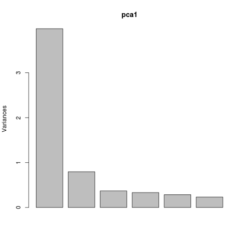
plot of chunk unnamed-chunk-3
pca1## Standard deviations:
## [1] 1.9952947 0.8924830 0.6077801 0.5767803 0.5350063 0.4837036
##
## Rotation:
## PC1 PC2 PC3 PC4 PC5
## Wingcrd -0.3617745 0.63271912 0.50662096 0.3258822675 -0.31354286
## Tarsus -0.4214011 0.07322892 -0.75093073 0.4624788082 -0.04496309
## Head -0.4459458 -0.19032228 0.01334900 -0.0002966949 -0.09030289
## Culmen -0.4099956 -0.39641642 0.38030979 0.2694261583 0.63356601
## Nalospi -0.4049720 -0.46052289 0.09015465 -0.3618441591 -0.58920702
## Wt -0.4007168 0.43457354 -0.16277793 -0.6902118236 0.37807906
## PC6
## Wingcrd -0.08725000
## Tarsus -0.19301118
## Head 0.86981428
## Culmen -0.23690880
## Nalospi -0.37106919
## Wt -0.06884131We could then use PCA1 (and maybe PCA2) as predictors in a regular lm() or glm(), to account for correlation between all the variables (this is often done for soil nutrient data).
We can visualize this information. The function biplot() depicts a PCA1 and PCA2 points for each sparrow and adds arrows corresponding to the direction and strength of each variable. In this case, one species is generally smaller than the other: hence all variables are smaller and the arrows all point one way. In other cases, the arrows will reflect much more variation in the data.
biplot(pca1)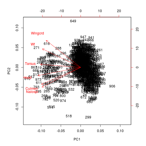
plot of chunk unnamed-chunk-4
We can also visualize these data using just points, and color-coding the species. In this instance, we need to use scores() to extract the pca axes from the object.
library(vegan)## Loading required package: permute
## Loading required package: lattice
## This is vegan 2.3-5plot(scores(pca1), col = dat$Species)
plot of chunk unnamed-chunk-5
And also change the plotting character according to sex.
plot(scores(pca1), col = dat$Species, pch = as.numeric(dat$Sex) )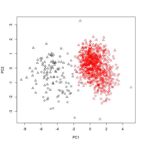
plot of chunk unnamed-chunk-6
The vegan and `labdsv' packages extend these analyses, to include more complex ordination methods, modelling one set of data (e.g., species x site) as a function of another (e.g., soils x site).
labdsv
load the package
library(labdsv)## Loading required package: mgcv
## Loading required package: nlme
## This is mgcv 1.8-12. For overview type 'help("mgcv-package")'.
## Loading required package: MASS
## Loading required package: cluster
##
## Attaching package: 'labdsv'
##
## The following object is masked from 'package:stats':
##
## densityExamine the vegetation data
It is a large species x site matrix of vegetation from Bryce Canyon, a famous US National Park.
library(labdsv)
veg <- read.table("../data/bryceveg.s", header = TRUE, row.names = 1)
dim(veg)
## [1] 160 169veg[1:10, 1:10]## junost ameuta arcpat arttri atrcan berfre ceamar cerled cermon
## bcnp__1 0 0.0 1.0 0 0 0 0.5 0 0
## bcnp__2 0 0.5 0.5 0 0 0 0.0 0 0
## bcnp__3 0 0.0 1.0 0 0 0 0.5 0 0
## bcnp__4 0 0.5 1.0 0 0 0 0.5 0 0
## bcnp__5 0 0.0 4.0 0 0 0 0.5 0 0
## bcnp__6 0 0.5 1.0 0 0 0 1.0 0 0
## bcnp__7 0 0.0 4.0 0 0 0 1.0 0 0
## bcnp__8 0 0.0 2.0 0 0 0 0.0 0 0
## bcnp__9 0 0.0 0.0 0 0 0 0.0 0 0
## bcnp_10 0 0.0 5.0 0 0 0 0.5 0 0
## chrdep
## bcnp__1 0
## bcnp__2 0
## bcnp__3 0
## bcnp__4 0
## bcnp__5 0
## bcnp__6 0
## bcnp__7 0
## bcnp__8 0
## bcnp__9 0
## bcnp_10 0PCA
Base R has two functions for principle components analysis
prcomp()computes a singular value decomposition and is used by labdsvprincomp()computes an eigenanalysis.
Labdsv uses its own function pca() as a wrapper for prcomp()
pca.1 <- pca(veg, cor = TRUE, dim = 10)
summary(pca.1, dim = 10)
## Importance of components:
## [,1] [,2] [,3] [,4]
## Standard deviation 3.65275545 2.77224856 2.66016722 2.5459628
## Proportion of Variance 0.07895043 0.04547552 0.04187272 0.0383546
## Cumulative Proportion 0.07895043 0.12442594 0.16629866 0.2046533
## [,5] [,6] [,7] [,8]
## Standard deviation 2.38617490 2.31459860 2.1179390 2.06713660
## Proportion of Variance 0.03369131 0.03170039 0.0265424 0.02528434
## Cumulative Proportion 0.23834456 0.27004496 0.2965874 0.32187170
## [,9] [,10]
## Standard deviation 1.90778099 1.85804579
## Proportion of Variance 0.02153626 0.02042801
## Cumulative Proportion 0.34340796 0.36383598Plot this PCA. The first panel shows the variance associated with each vector, and the second shows the cumulative variance as a fraction of the total.
par(mfrow = c(1,2))
varplot.pca(pca.1)
## Hit Return to Continue
Species loadings
head(pca.1$loadings)## PC1 PC2 PC3 PC4 PC5
## junost 0.043840911 0.02118713 0.05524806 -0.01840697 -0.09753036
## ameuta -0.078493527 -0.02588778 -0.03481203 0.02929972 -0.03648105
## arcpat -0.156746871 -0.05938271 -0.07409708 -0.02810666 0.10296989
## arttri 0.026890004 0.21899596 0.14744798 0.02121300 -0.15431408
## atrcan 0.024513563 0.20333835 0.14396096 0.01597171 -0.15396256
## berfre -0.001079674 0.07306636 0.08236608 -0.07331151 -0.03334877
## PC6 PC7 PC8 PC9 PC10
## junost -0.03957741 -0.053221404 0.09677946 -0.09138364 0.08187130
## ameuta 0.01415789 -0.013711349 -0.06409484 0.02415719 -0.03703925
## arcpat -0.02794704 -0.001833523 0.05705832 -0.13834423 -0.02259668
## arttri -0.08617191 -0.025668792 0.15771245 -0.11744406 -0.03912206
## atrcan -0.09461440 -0.028068846 0.15204417 -0.07970031 -0.04658211
## berfre -0.02008131 -0.064619236 -0.05169453 -0.07257582 -0.08039237Plot scores
head(pca.1$scores)## PC1 PC2 PC3 PC4 PC5 PC6
## bcnp__1 -2.110215 0.09732253 -0.22470551 1.3316310 -0.4293049 -0.06088433
## bcnp__2 -3.155726 -1.44154295 -1.31540270 3.2960477 -0.9330680 -0.54655498
## bcnp__3 -2.356623 -0.99119732 -0.74045845 2.4512855 -0.8586722 -0.35849801
## bcnp__4 -1.852786 0.01964674 -0.04842751 0.7798660 0.3324656 -0.43264173
## bcnp__5 -3.885253 -1.22546353 -1.39372043 0.8798713 0.7824252 -0.39229854
## bcnp__6 -2.859971 -0.22638760 -0.41159427 1.3959822 -0.5067462 -0.10774144
## PC7 PC8 PC9 PC10
## bcnp__1 0.35154684 -0.73911742 1.1908025 -0.0740778
## bcnp__2 0.07992399 1.38683706 2.1974011 -3.0121350
## bcnp__3 0.04587622 0.72342469 1.8475835 -1.5878440
## bcnp__4 0.34610039 -0.09052725 0.7390983 0.3082807
## bcnp__5 0.61498142 1.20647359 -1.5027409 -0.5199233
## bcnp__6 0.07613708 -0.68030216 0.8709883 -0.4689155Using plot() on a pca object calls plot.pca(), and plots the first two axes by default.
plot(pca.1, title = "Bryce Canyon") 
Environmental analysis
First, center the species abundances around their means and standardize their variance
veg.center <- apply(veg, 2, function(x){(x - mean(x)) / sd(x)} )

# or:
veg.center <- scale(veg, center = TRUE, scale = TRUE)
Then, load the environmental variables
site <- read.table("../data/brycesit.s", header = TRUE)
head(site)
## labels annrad asp av depth east elev grorad north pos quad
## 1 50001 241 30 1.00 deep 390 8720 162 4100 ridge pc
## 2 50002 222 50 0.96 shallow 390 8360 156 4100 mid_slope pc
## 3 50003 231 50 0.96 shallow 390 8560 159 4100 mid_slope pc
## 4 50004 254 360 0.93 shallow 390 8660 166 4100 ridge pc
## 5 50005 232 300 0.48 shallow 390 8480 159 4100 up_slope pc
## 6 50006 216 330 0.76 shallow 390 8560 155 4100 mid_slope pc
## slope
## 1 9
## 2 2
## 3 2
## 4 0
## 5 2
## 6 2Modelling
We will model elevation as a function of previous PCA scores.
elev.pca.glm <- glm(site$elev ~ pca.1$scores[,1] + pca.1$scores[,2])
summary(elev.pca.glm)
##
## Call:
## glm(formula = site$elev ~ pca.1$scores[, 1] + pca.1$scores[,
## 2])
##
## Deviance Residuals:
## Min 1Q Median 3Q Max
## -1123.26 -361.72 19.48 396.99 964.19
##
## Coefficients:
## Estimate Std. Error t value Pr(>|t|)
## (Intercept) 7858.56 39.89 196.982 < 2e-16 ***
## pca.1$scores[, 1] -56.33 10.96 -5.142 8.01e-07 ***
## pca.1$scores[, 2] -105.72 14.44 -7.323 1.19e-11 ***
## ---
## Signif. codes: 0 '***' 0.001 '**' 0.01 '*' 0.05 '.' 0.1 ' ' 1
##
## (Dispersion parameter for gaussian family taken to be 254655.1)
##
## Null deviance: 60370369 on 159 degrees of freedom
## Residual deviance: 39980847 on 157 degrees of freedom
## AIC: 2450.7
##
## Number of Fisher Scoring iterations: 2Plot the model
require(akima) # to load the interp() function## Loading required package: akima## Warning in library(package, lib.loc = lib.loc, character.only = TRUE,
## logical.return = TRUE, : there is no package called 'akima'plot(pca.1 )
# add model contour lines, using interp() to interpolate grid of values
contour(interp(pca.1$scores[,1], pca.1$scores[,2], fitted(elev.pca.glm)),
    add = TRUE, col = 2, labcex = 0.8)
## Error in contour(interp(pca.1$scores[, 1], pca.1$scores[, 2], fitted(elev.pca.glm)), : could not find function "interp"# add real contour lines:
contour(interp(pca.1$scores[,1], pca.1$scores[,2], site$elev), add = TRUE, col = 3)## Error in contour(interp(pca.1$scores[, 1], pca.1$scores[, 2], site$elev), : could not find function "interp"It looks like the model may be non-linear, so try ...
elev.pca2.glm <- glm( site$elev ~ pca.1$scores[,1] + I(pca.1$scores[,1]^2) + pca.1$scores[,2] + I(pca.1$scores[,2]^2) )
summary(elev.pca2.glm)
##
## Call:
## glm(formula = site$elev ~ pca.1$scores[, 1] + I(pca.1$scores[,
## 1]^2) + pca.1$scores[, 2] + I(pca.1$scores[, 2]^2))
##
## Deviance Residuals:
## Min 1Q Median 3Q Max
## -1222.55 -323.09 60.59 258.48 930.73
##
## Coefficients:
## Estimate Std. Error t value Pr(>|t|)
## (Intercept) 7628.726 64.476 118.320 < 2e-16 ***
## pca.1$scores[, 1] -117.975 17.264 -6.834 1.78e-10 ***
## I(pca.1$scores[, 1]^2) 20.813 3.495 5.956 1.67e-08 ***
## pca.1$scores[, 2] -65.096 14.337 -4.540 1.12e-05 ***
## I(pca.1$scores[, 2]^2) -6.040 3.050 -1.980 0.0494 *
## ---
## Signif. codes: 0 '***' 0.001 '**' 0.01 '*' 0.05 '.' 0.1 ' ' 1
##
## (Dispersion parameter for gaussian family taken to be 203030.2)
##
## Null deviance: 60370369 on 159 degrees of freedom
## Residual deviance: 31469682 on 155 degrees of freedom
## AIC: 2416.4
##
## Number of Fisher Scoring iterations: 2Check if model is significantly better
anova( elev.pca.glm, elev.pca2.glm, test="Chi" )## Analysis of Deviance Table
##
## Model 1: site$elev ~ pca.1$scores[, 1] + pca.1$scores[, 2]
## Model 2: site$elev ~ pca.1$scores[, 1] + I(pca.1$scores[, 1]^2) + pca.1$scores[,
## 2] + I(pca.1$scores[, 2]^2)
## Resid. Df Resid. Dev Df Deviance Pr(>Chi)
## 1 157 39980847
## 2 155 31469682 2 8511165 7.889e-10 ***
## ---
## Signif. codes: 0 '***' 0.001 '**' 0.01 '*' 0.05 '.' 0.1 ' ' 1Plot the new model
plot(pca.1)
contour(interp(pca.1$scores[,1], pca.1$scores[,2], fitted(elev.pca2.glm)), add = TRUE, col = 2)## Error in contour(interp(pca.1$scores[, 1], pca.1$scores[, 2], fitted(elev.pca2.glm)), : could not find function "interp"PCA operates on a correlation or covariance matrix, and that these structures are really not appropriate for vegetation data that spans a large amount of environmental variability, or that exhibits much beta diversity.
Look over the LABDSV website for further examples of ordination.