Intro to R for Biologists
Class 1 - Guided R session
Simon Queenborough
Evolution, Ecology & Organismal Biology, OSU
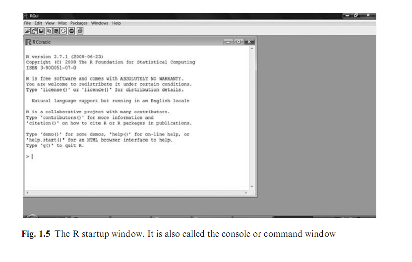
The R window
Basic arithmetic
R input (copy and paste into R window)
2 + 2 # R output (below)
## [1] 4
2 + 2
## [1] 4
2 + 2
## [1] 4
Basic arithmetic
log(2)
## [1] 0.6931
log(10)
## [1] 2.303
Basic arithmetic
Fails:
2 + 2*w
Basic arithmetic
Need to define 'w'
w <- 10
2 + 2 * w
## [1] 22
Example 1
library(lattice)
dat <- read.table('data/ISIT.txt',header=TRUE,sep='\t')
xyplot(Sources~SampleDepth|factor(Station),data=dat,
xlab='Sample Depth',ylab='Sources',
strip=function(bg='white', ...)
strip.default(bg='white',...),
panel=function(x,y){
panel.grid(h=-1,v=2)
I1=order(x)
llines(x[I1],y[I1],col=1)})
Example 1

Writing R Code
It is impossible to remember all the commands and programs!
Therefore, VERY important to:
- Write SIMPLE code
- Write many comments describing what the code does:
# a comment
Example 1 with comments
# load libraries/packages
library(lattice)
# read in data
dat <- read.table('data/ISIT.txt',header=TRUE,sep='\t')

# Start plotting:
#   - plot Sources as a function of SampleDepth,
#   - use a panel for each Station
#   - use colour black (col = 1), and
#   - specify x and y labels (xlab and ylab).
#   - use white background in the boxes that contain station labels

xyplot(Sources~SampleDepth|factor(Station),data=dat,
xlab='Sample Depth',ylab='Sources',
strip=function(bg='white', ...)
strip.default(bg='white',...),
panel=function(x,y){
  # avoid grid lines
  # avoid spaghetti plots
  # plot data as lines (in black)
panel.grid(h=-1,v=2)
I1=order(x)
llines(x[I1],y[I1],col=1)})
More recommendations
- Use spaces to indicate groups of commands
- Use spaces around text
Example 1 with comments and spaces
# load libraries/packages
library(lattice)
# read in data
dat <- read.table('data/ISIT.txt', header = TRUE, sep = '\t')

# Start plotting:
#   - plot Sources as a function of SampleDepth,
#   - use a panel for each Station
#   - use colour black (col = 1), and
#   - specify x and y labels (xlab and ylab).
#   - use white background in the boxes that contain station labels
Example 1 with comments and spaces and nesting
xyplot(Sources ~ SampleDepth | factor(Station), data = dat,
      xlab = 'Sample Depth', ylab = 'Sources',
      strip = function(bg = 'white', ...)
      strip.default(bg = 'white', ...),
      panel = function(x, y){
        # avoid grid lines
        # avoid spaghetti plots
        # plot data as lines (in black)
        panel.grid(h = -1, v = 2)
        I1 = order(x)
        llines(x[I1], y[I1], col = 1)
      } # close panel()
) # close xyplot
Coding Style Guides
Good style is important because while your code only has one author, it will usually have multiple readers
Hadley Wickham
Text editors
Text editors use unformatted plain text with no hidden characters or code. Thus, what you paste in to R is what runs. Most text editors also have nice syntax highlighting. Word processors such as MS-Word contain formatted text.
Common ones:
Hard-core
NEVER, NEVER M$-Word/equivalent!
Graphics in R
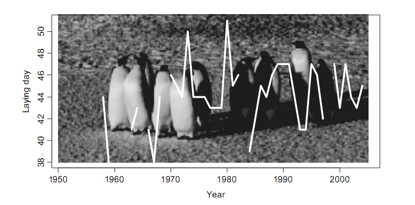
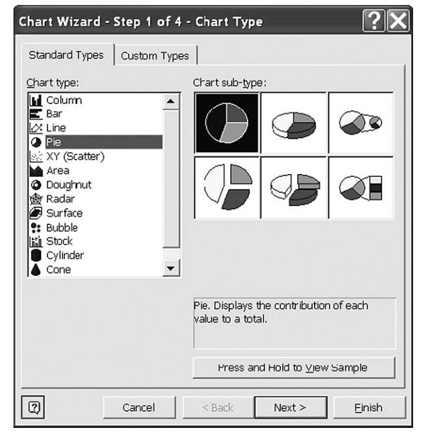
It is possible to do graphics that would maybe be faster in Excel ...
- if you only have to do them once, and
- if they are not too complex.
The nightmare of many statisticians!
Packages
- ~ ‘library’
- A collection of previously programmed functions
- Equivalent to many commercial software: e.g. Multivariate stats: vegan = PCORD, CANOCO etc.
- Need to download from CRAN:
install.packages("foo")
library(foo) # or
require(foo)
Quiting R
q()
Save workspace? Usually not.
Better to save commands as text files
rm(list = ls(all = TRUE))