FES 720 Introduction to R

Working with Data in R

FES 720: Intro to R

A. Types of Data

B. Getting Data into R

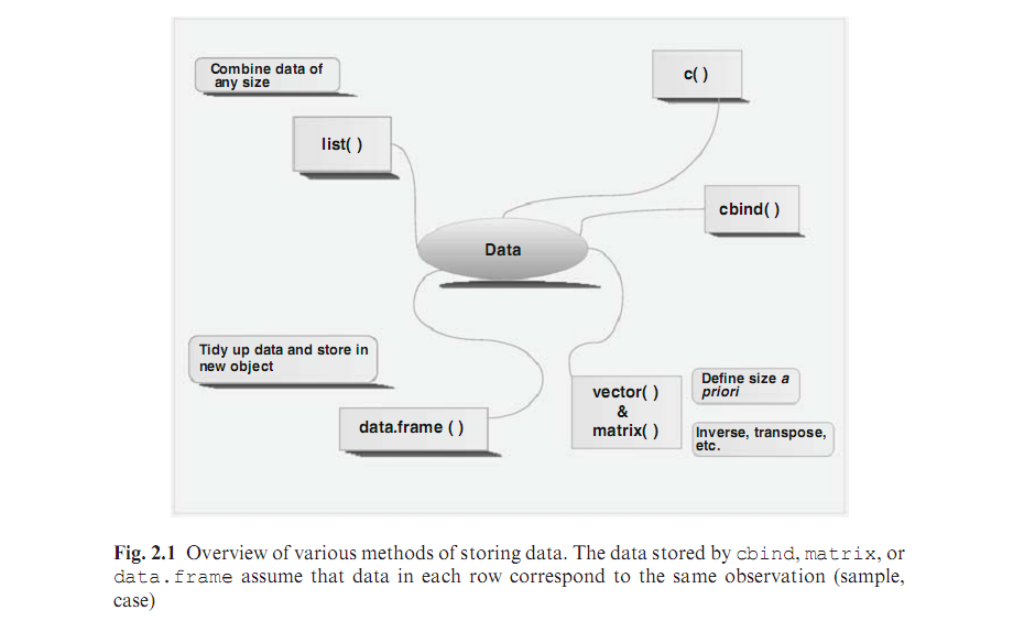
There are various ways to import data into R.

Entering data by hand
Entering data with c()
Combining variables: c(), cbind(), rbind()
Functions vector(), matrix(), list(), data.frame()
But better to enter it outside of R in a spreadsheet

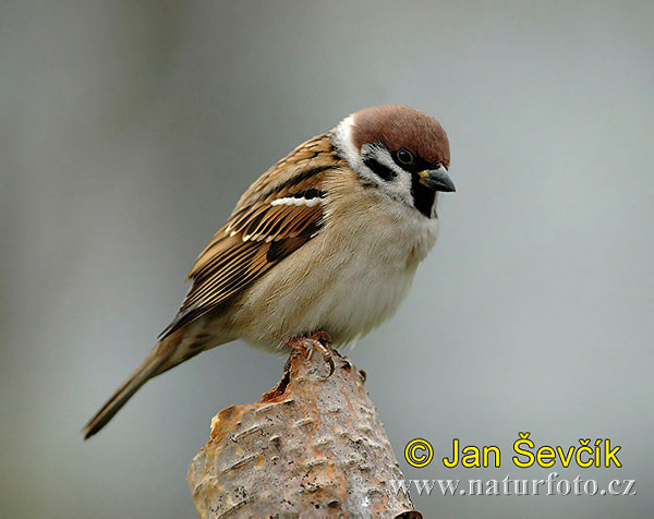
We will practice on several measurements of sparrows.

B.1. Entering data by hand

You can enter every number as an object:

a <- 59
b <- 55
c <- 53.5
d <- 55
e <- 52.5

Which will then return each object’s value

But the names of these objects (eg. a) are not very useful; it is much better to give them useful names.

Wing1 <- 59
Wing2 <- 55
Wing3 <- 53.5
Wing4 <- 55
Wing5 <- 52.5

These objects can then be used in any other calculation.

sqrt(Wing1)
2 * Wing1
Wing1 + Wing2
Wing1 + Wing2 + Wing3 + Wing4 + Wing5
(Wing1 + Wing2 + Wing3 + Wing4 + Wing5) / 5

But R does not save the results of calculations unless they are named objects too

SQ.wing1 <- sqrt(Wing1)
Mul.W1 <- 2 * Wing1
Sum.12 <- Wing1 + Wing2
SUM12345 <- Wing1 + Wing2 + Wing3 + Wing4 + Wing5
Av <- (Wing1 + Wing2 + Wing3 + Wing4 + Wing5) / 5

B.2. Entering data with concatenate: c()

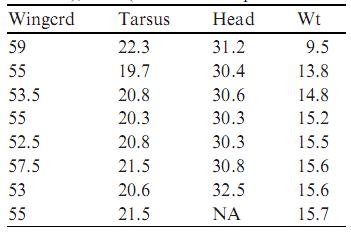
Wingcrd <- c(59, 55, 53.5, 55, 52.5, 57.5, 53, 55)

We can then pull out elements of Wingcrd with square brackets: []

Wingcrd[1]
Wingcrd [1:5]
Wingcrd [-2]

Various functions to calculate summary data from vectors are built in to R

S.win <- sum(Wingcrd)
S.win

mean(Wingcrd)
max(Wingcrd)
min(Wingcrd)
median(Wingcrd)
var(Wingcrd)
sd(Wingcrd)

We can enter the other data in the same way

Tarsus <- c(22.3, 19.7, 20.8, 20.3, 20.8, 21.5, 20.6, 21.5)
Head <- c(31.2, 30.4, 30.6, 30.3, 30.3, 30.8, 32.5, NA)
Wt <- c(9.5, 13.8, 14.8, 15.2, 15.5, 15.6, 15.6, 15.7)

B.3. Combining variables: c(), cbind(), rbind()

In a vector

BirdData <- c(Wingcrd, Tarsus, Head, Wt)

Create another column to identify the variables

Id <- c(1, 1, 1, 1, 1, 1, 1, 1, 2, 2, 2, 2, 2, 2, 2,
     2, 3, 3, 3, 3, 3, 3, 3, 3, 4, 4, 4, 4, 4, 4, 4, 4)

Various other (simpler) ways

Id <- rep(c(1, 2, 3, 4), each = 8)

Id <- rep(1:4, each = 8)

Id <- seq(from = 1, to = 4, by = 1)

a <- seq(from = 1, to = 4, by = 1)
Id <- rep(a, each = 8)

There are often a number of ways to carry out the same task in R.

Different analyses may require different data formats e.g., a table vs. a vector.

Unite data by columns: cbind()

Z <- cbind(Wingcrd, Tarsus, Head, Wt)

Index Z using [,]

Z[,1] # column 1
Z[1,] # row 1

Z[1:8, 1]

Z[1, 1]
Z[,2:3]

These elements can be assigned to other variables

X <- Z[4, 4]
Y <- Z[,4]
W <- Z[,-3]
D <- Z[, c(1, 3, 4)]
E <- Z[, c(-1, -3)]

dimensions of Z

n <- dim(Z)

z.row <- dim(Z)[1]

using `rbind()`

Z2 <- rbind(Wingcrd, Tarsus, Head, Wt)

B.4. Function: vector()

Generates an empty vector. It is useful to define how many elements will be in the vector e.g. in loops

W <- vector(length = 8)
w   # NB: case sensitive!

Fill the vector

W[1] <- 59
W[2] <- 55
W[3] <- 53.5
W[4] <- 55
W[5] <- 52.5
W[6] <- 57.5
W[7] <- 53
W[8] <- 55
W

Pull out elements

W[1]
W[1 : 4]
W[2 : 6]
W[-2]
W[c (1, 3, 5)]
W[9] # there is no w[9]!

B.5. Uniting data with matrix()

Instead of generating 4 vectors with length 8, we can generate a matrix of dimensions 8 by 4.

Dmat <- matrix(nrow = 8, ncol = 4)

And then fill the matrix by column

Dmat[, 1] <- c(59, 55, 53.5, 55, 52.5, 57.5, 53, 55)
Dmat[, 2] <- c(22.3, 19.7, 20.8, 20.3, 20.8, 21.5,
                 20.6, 21.5)
Dmat[, 3] <- c(31.2, 30.4, 30.6, 30.3, 30.3, 30.8,
                 32.5, NA)
Dmat[, 4] <- c(9.5, 13.8, 14.8, 15.2, 15.5, 15.6,
                 15.6, 15.7)

Dmat # matrix without names

B.6. Functions: colnames(), rownames()

colnames(Dmat) <- c("Wingcrd", "Tarsus", "Head", "Wt")
Dmat

We can fill the matrix element by element, but takes a rather long time!

Dmat[1, 1] <- 59.0
Dmat[1, 2] <- 22.3 

Rather, we can combine existing data.

Dmat2 <- as.matrix(cbind(Wingcrd, Tarsus, Head, Wt))
Dmat2

NB: in R there are many ways to do the same thing. Certain functions only accept matrices, not data.frames.

other functions on matrices:

is.matrix(Dmat2)    # confirm it is a matrix
t(Dmat2)            # transpose
#Dmat %*% Dmat2      # matrix multiplication  
#solve(Dmat2)        # inverse

B.7. Function: data.frame()

use:

combine variables of equal length
can combine vectors of numbers, character strings, and factors (nominal or categorical) variables in the same object
almost all results produced by functions are in the form of lists

Dfrm <- data.frame(WC = Wingcrd, TS = Tarsus, HD = Head, W = Wt)

We can do calculations and include the result in the data frame:

Dfrm <- data.frame(WC = Wingcrd, TS = Tarsus, HD = Head, W=Wt, Wsq = sqrt(Wt))

Note that Wt != W

rm(Wt)
Wt

# but Dfrm$w still exists:
Dfrm$W

B.8. Function list()

Until now, each row of data was equal to a single unit of sampling

A list is an object within which you can place unrelated objects, such as vectors, matrices, or characters. Each row, therefore, is not one sample unit.

For example, take …

# ... a vector ...
x1 <- c(1, 2, 3)

# ... a factor ...
x2 <- c("a", "b", "c", "d")

# ... a scalar (vector of size 1) ...
x3 <- 3

# ... and a matrix.
x4 <- matrix(nrow = 2, ncol = 2)
x4[,1] <- c(1, 2)
x4[,2] <- c( 3, 4)

And combine all 5 objects in a list

Y <- list(x1 = x1, x2 = x2, x3 = x3, x4 = x4)

Y

Function outputs are usually lists

# e.g. linear regression
M <- lm(WC ~ W, data = Dfrm)
names(M)

# a list!:
M$coefficients

C. Importing Data

It is much easier to import data from other programmes than enter them again by hand into R.

Importing data is the most difficult thing in R (at least in the beginning…).

Overview

Enter the data in a spreadsheet (Excel, Gnumeric, OpenOffice Calc)
Export the data as tab-delimited text file
Close the spreadsheet
setwd("my/file/locations/") to working directory
Import the data into R with read.table(), read.cvs() or similar:

dat.sparrows <- read.table(file = "sparrow.txt", header = TRUE)

(other functions can import data directly from Excel etc. NOT RECOMMENDED.)

Details

1. Enter data in spreadsheet (e.g. gnumeric, OpenOffice Calc, Excel).

‘NA’ for missing data
First row = names of variables
First column = unit of sampling
Names without spaces, #, etc.
No # or ‘ in the file (comment sign in R)

2. Copy and paste into text editor

Save as foo.txt file
Copy and paste the file address
[WINDOWS] Change the \ to: \\ or /
[WINDOWS] Include spaces in file hierarchy: /My Documents/ as is

5. Import the data

Commas or periods?

Excel uses . or , to separate decimals, depending on location
If the file was made in a computer with ,, you must include the argument: read.table("filename.txt", dec= ",", ...).

dat <- read.table(file = "sparrows.txt", header = TRUE)
dat <- read.table(file = "sparrows.txt", header = TRUE, dec = ",")
dat <- read.csv(file   = "sparrows.csv", header = TRUE)

Did that data import correctly?

dat <- read.table(file = "data/sparrows.txt", header = TRUE)
summary(dat)

    Wingcrd          Tarsus           Head             Wt       
 Min.   :52.50   Min.   :19.70   Min.   :30.30   Min.   : 9.50  
 1st Qu.:53.38   1st Qu.:20.52   1st Qu.:30.35   1st Qu.:14.55  
 Median :55.00   Median :20.80   Median :30.60   Median :15.35  
 Mean   :55.06   Mean   :20.94   Mean   :30.87   Mean   :14.46  
 3rd Qu.:55.62   3rd Qu.:21.50   3rd Qu.:31.00   3rd Qu.:15.60  
 Max.   :59.00   Max.   :22.30   Max.   :32.50   Max.   :15.70  
                                 NA's   :1                      

D. Obtaining Data Remotely

Function: read.table()

dat <- read.table(file = "http://www.simonqueenborough.info/R/data/sparrows.txt")

HTML tables in webpages

library(XML)
dat <- readHTMLTable()

Function: url()

dat <- url()

Updated: 2017-10-01